Define a connection function with a field output

In this example, we define a function which has a vector input and a field output. The goal of this example is to show how to use the PointToFieldConnection to combine two functions. A detailed explanation of the model is presented here.

Define the model

from __future__ import print_function
import openturns as ot
import openturns.viewer as viewer
from matplotlib import pylab as plt
import numpy as np
ot.Log.Show(ot.Log.NONE)

We first define the time grid associated with the model.

tmin=0.0 # Minimum time
tmax=12. # Maximum time
gridsize=100 # Number of time steps
mesh = ot.IntervalMesher([gridsize-1]).build(ot.Interval(tmin, tmax))

vertices = mesh.getVertices()

Creation of the input distribution.

distZ0 = ot.Uniform(100.0, 150.0)
distV0 = ot.Normal(55.0, 10.0)
distM = ot.Normal(80.0, 8.0)
distC = ot.Uniform(0.0, 30.0)
distribution = ot.ComposedDistribution([distZ0, distV0, distM, distC])

dimension = distribution.getDimension()
dimension

Out:

4

Then we define the Python function which computes the altitude at each time value. This function has 5 inputs: z0, v0, m, c and zmin.

def AltiFunc(X):
    g  = 9.81
    z0 = X[0]
    v0 = X[1]
    m  = X[2]
    c  = X[3]
    zmin  = X[4]
    tau = m / c
    vinf = - m * g / c
    t = np.array(vertices)
    z = z0 + vinf * t + tau * (v0 - vinf) * (1 - np.exp( - t / tau))
    z = np.maximum(z,zmin)
    return [[zeta[0]] for zeta in z]

outputDimension = 1
altitudeWithFiveInputs = ot.PythonPointToFieldFunction(5, mesh, outputDimension, AltiFunc)

Restrict the number of inputs

We define a function which has 4 inputs and 5 outputs: the 5th ouput zmin is set to zero.

projectionFunction = ot.SymbolicFunction(["z0", "v0", "m", "c"], ["z0", "v0", "m", "c", "0.0"])

Then we use the PointToFieldConnection to create a function which has 4 inputs and returns the output field.

altitudeWithFourInputs = ot.PointToFieldConnection(altitudeWithFiveInputs, projectionFunction)

Sample trajectories

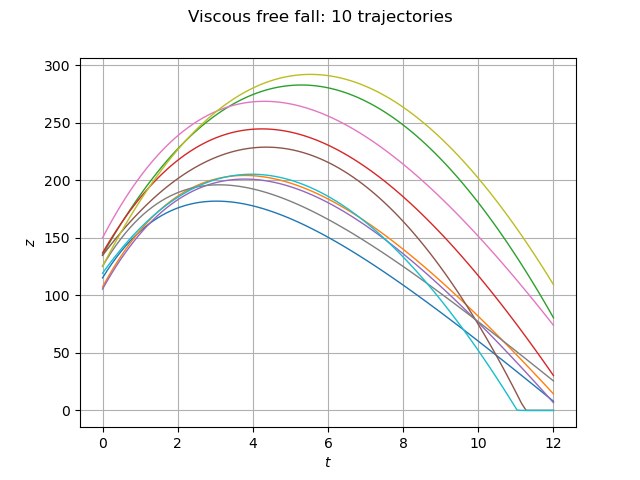
In order to sample trajectories, we use the getSample method of the input distribution and apply the field function.

size = 10
inputSample = distribution.getSample(size)
outputSample = altitudeWithFourInputs(inputSample)

Draw some curves.

graph = outputSample.drawMarginal(0)
graph.setTitle('Viscous free fall: %d trajectories' % (size))
graph.setXTitle(r'$t$')
graph.setYTitle(r'$z$')
view = viewer.View(graph)
plt.show()