Note
Click here to download the full example code
Viscous free fall: metamodel of a field function
In this example, we present how to create the metamodel of a field function. This examples considers the free fall model. We first compute the Karhunen-Loève decomposition of a sample of trajectories. Then we create a create a polynomial chaos which takes the inputs and returns the KL decomposition modes as outputs. Finally, we create a metamodel by combining the KL decomposition and the polynomial chaos.
Define the model
from __future__ import print_function
import openturns as ot
import numpy as np
import openturns.viewer as viewer
from matplotlib import pylab as plt
ot.Log.Show(ot.Log.NONE)
We first define the time grid associated with the model.
tmin=0.0 # Minimum time
tmax=12. # Maximum time
gridsize=100 # Number of time steps
mesh = ot.IntervalMesher([gridsize-1]).build(ot.Interval(tmin, tmax))
vertices = mesh.getVertices()
Creation of the input distribution.
distZ0 = ot.Uniform(100.0, 150.0)
distV0 = ot.Normal(55.0, 10.0)
distM = ot.Normal(80.0, 8.0)
distC = ot.Uniform(0.0, 30.0)
distribution = ot.ComposedDistribution([distZ0, distV0, distM, distC])
dimension = distribution.getDimension()
dimension
Out:
4
Then we define the Python function which computes the altitude at each time value. In order to compute all altitudes with a vectorized evaluation, we first convert the vertices into a Numpy array and use the Numpy functions`exp` and maximum: this increases the evaluation performance of the script.
def AltiFunc(X):
    g  = 9.81
    z0 = X[0]
    v0 = X[1]
    m  = X[2]
    c  = X[3]
    tau = m / c
    vinf = - m * g / c
    t = np.array(vertices)
    z = z0 + vinf * t + tau * (v0 - vinf) * (1 - np.exp( - t / tau))
    z = np.maximum(z,0.)
    return [[zeta[0]] for zeta in z]
In order to create a Function from this Python function, we use the PythonPointToFieldFunction class. Since the altitude is the only output field, the third argument outputDimension is equal to 1. If we had computed the speed as an extra output field, we would have set 2 instead.
outputDimension = 1
alti = ot.PythonPointToFieldFunction(dimension, mesh, outputDimension, AltiFunc)
Compute a training sample.
size = 2000
ot.RandomGenerator.SetSeed(0)
inputSample = distribution.getSample(size)
outputSample = alti(inputSample)
Compute the KL decomposition of the output
algo = ot.KarhunenLoeveSVDAlgorithm(outputSample, 1.0e-6)
algo.run()
KLResult = algo.getResult()
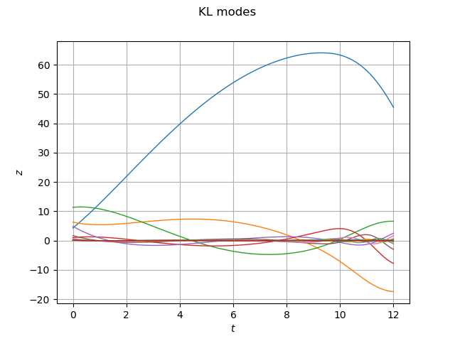
scaledModes = KLResult.getScaledModesAsProcessSample()
graph = scaledModes.drawMarginal(0)
graph.setTitle('KL modes')
graph.setXTitle(r'$t$')
graph.setYTitle(r'$z$')
view = viewer.View(graph)
We create the postProcessingKL function which takes coefficients of the the K.-L. modes as inputs and returns the trajectories.
karhunenLoeveLiftingFunction = ot.KarhunenLoeveLifting(KLResult)
The project method computes the projection of the output sample (i.e. the trajectories) onto the K.-L. modes.
outputSampleChaos = KLResult.project(outputSample)
We limit the sampling size of the Lilliefors selection in order to reduce the computational burden.
ot.ResourceMap.SetAsUnsignedInteger("FittingTest-LillieforsMaximumSamplingSize", 1)
We create a polynomial chaos metamodel which takes the input sample and returns the K.-L. modes.
algo = ot.FunctionalChaosAlgorithm(inputSample, outputSampleChaos)
algo.run()
chaosMetamodel = algo.getResult().getMetaModel()
The final metamodel is a composition of the KL lifting function and the polynomial chaos metamodel. In order to combine these two functions, we use the PointToFieldConnection class.
metaModel = ot.PointToFieldConnection(karhunenLoeveLiftingFunction, chaosMetamodel)
Validate the metamodel
Create a validation sample.
size = 10
validationInputSample = distribution.getSample(size)
validationOutputSample = alti(validationInputSample)
graph = validationOutputSample.drawMarginal(0)
graph.setColors(['red'])
graph2 = metaModel(validationInputSample).drawMarginal(0)
graph2.setColors(['blue'])
graph.add(graph2)
graph.setTitle('Model/metamodel comparison')
graph.setXTitle(r'$t$')
graph.setYTitle(r'$z$')
view = viewer.View(graph)
plt.show()
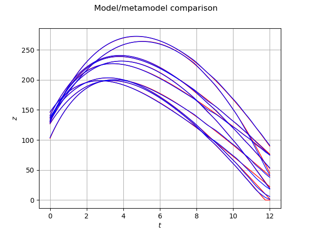
We see that the blue trajectories (i.e. the metamodel) are close to the red trajectories (i.e. the validation sample). This shows that the metamodel is quite accurate. However, we observe that the trajectory singularity that occurs when the object touches the ground (i.e. when  is equal to zero), makes the metamodel less accurate.
Total running time of the script: ( 0 minutes 27.279 seconds)