Note
Click here to download the full example code
Create a linear least squares model
In this example we are going to create a global approximation of a model response using a linear function:

Here
![h(x) = [cos(x_1 + x_2), (x2 + 1)* e^{x_1 - 2* x_2}]](../../_images/math/722482215db17f773b070e7ee65e52004ce741ec.svg)
from __future__ import print_function
import openturns as ot
import openturns.viewer as viewer
from matplotlib import pylab as plt
ot.Log.Show(ot.Log.NONE)

# Prepare an input sample
x  = [[0.5,0.5], [-0.5,-0.5], [-0.5,0.5], [0.5,-0.5]]
x += [[0.25,0.25], [-0.25,-0.25], [-0.25,0.25], [0.25,-0.25]]
Compute the output sample from the input sample and a function
formulas = ['cos(x1 + x2)', '(x2 + 1) * exp(x1 - 2 * x2)']
model = ot.SymbolicFunction(['x1', 'x2'], formulas)
y = model(x)
create a linear least squares model
algo = ot.LinearLeastSquares(x, y)
algo.run()
get the linear term
algo.getLinear()
[[ 9.93014e-17 0.998189 ]
[ 0 -0.925648 ]]
get the constant term
algo.getConstant()
[0.854471,1.05305]
get the metamodel
responseSurface = algo.getMetaModel()
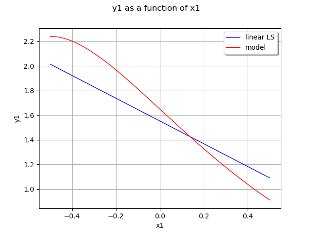
plot 2nd output of our model with x1=0.5
graph = ot.ParametricFunction(responseSurface, [0], [0.5]).getMarginal(1).draw(-0.5, 0.5)
graph.setLegends(['linear LS'])
curve = ot.ParametricFunction(model, [0], [0.5]).getMarginal(1).draw(-0.5, 0.5).getDrawable(0)
curve.setColor('red')
curve.setLegend('model')
graph.add(curve)
graph.setLegendPosition('topright')
view = viewer.View(graph)
plt.show()
Total running time of the script: ( 0 minutes 0.079 seconds)