Taylor approximations

In this example we are going to build a local approximation of a model using the taylor decomposition:

Here is the decomposition at the first order:

Here .

from __future__ import print_function
import openturns as ot
import openturns.viewer as viewer
from matplotlib import pylab as plt
ot.Log.Show(ot.Log.NONE)

# prepare some data
formulas = ['cos(x1 + x2)', '(x2 + 1) * exp(x1 - 2 * x2)']
model = ot.SymbolicFunction(['x1', 'x2'], formulas)

# center of the approximation
x0 = [-0.4, -0.4]

# drawing bounds
a=-0.4
b=0.0

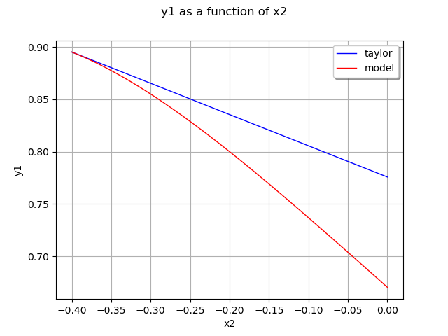
create a linear (first order) Taylor approximation

algo = ot.LinearTaylor(x0, model)
algo.run()
responseSurface = algo.getMetaModel()

plot 2nd output of our model with x1=x0_1

graph = ot.ParametricFunction(responseSurface, [0], [x0[1]]).getMarginal(1).draw(a, b)
graph.setLegends(['taylor'])
curve = ot.ParametricFunction(model, [0], [x0[1]]).getMarginal(1).draw(a, b).getDrawable(0)
curve.setColor('red')
curve.setLegend('model')
graph.add(curve)
graph.setLegendPosition('topright')
view = viewer.View(graph)

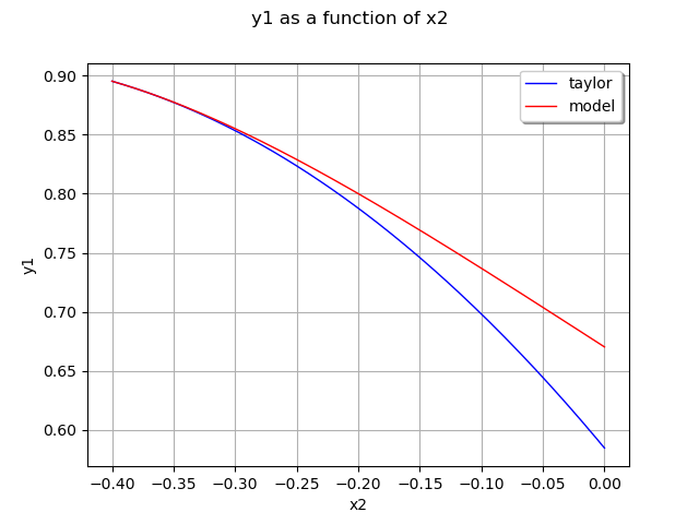
Here is the decomposition at the second order:

create a quadratic (2nd order) Taylor approximation

algo = ot.QuadraticTaylor(x0, model)
algo.run()
responseSurface = algo.getMetaModel()

plot 2nd output of our model with x1=x0_1

graph = ot.ParametricFunction(responseSurface, [0], [x0[1]]).getMarginal(1).draw(a, b)
graph.setLegends(['taylor'])
curve = ot.ParametricFunction(model, [0], [x0[1]]).getMarginal(1).draw(a, b).getDrawable(0)
curve.setColor('red')
curve.setLegend('model')
graph.add(curve)
graph.setLegendPosition('topright')
view = viewer.View(graph)
plt.show()