Note
Click here to download the full example code
Create a polynomial chaos metamodel by integration on the cantilever beam
In this example, we create a polynomial chaos metamodel by integration on the cantilever beam example.
In order to do this, we use the GaussProductExperiment class.
import openturns as ot
import openturns.viewer as viewer
from matplotlib import pylab as plt
ot.Log.Show(ot.Log.NONE)
We first load the model from the usecases module :
from openturns.usecases import cantilever_beam as cantilever_beam
cb = cantilever_beam.CantileverBeam()
In this example we consider all marginals independent. They are defined in the CantileverBeam data class as well as an independent distribution :
dist_E = cb.E
dist_F = cb.F
dist_L = cb.L
dist_I = cb.I
myDistribution = cb.independentDistribution
dim_input = cb.dim # dimension of the input
dim_output = 1 # dimension of the output
We load the model :
g = cb.model
Create a polynomial chaos decomposition
We create the multivariate polynomial basis by tensorization of the univariate polynomials and the default linear enumerate rule.
multivariateBasis = ot.OrthogonalProductPolynomialFactory([dist_E, dist_F, dist_L, dist_I])
Generate an training sample of size N with MC simulation.
N = 50 # size of the experimental design
inputTrain = myDistribution.getSample(N)
outputTrain = g(inputTrain)
We select the FixedStrategy truncation rule, which corresponds to using the first P polynomials of the polynomial basis. In this case, we select P using the getStrataCumulatedCardinal method, so that all polynomials with total degree lower or equal to 5 are used.
totalDegree = 5
enumfunc = multivariateBasis.getEnumerateFunction()
P = enumfunc.getStrataCumulatedCardinal(totalDegree)
adaptiveStrategy = ot.FixedStrategy(multivariateBasis, P)
adaptiveStrategy
class=FixedStrategy derived from class=AdaptiveStrategyImplementation maximumDimension=126
We see that the number of polynomials is equal to 126. This will lead to the computation of 126 coefficients.
We now set the method used to compute the coefficients; we select the integration method.
We begin by getting the standard measure associated with the multivariate polynomial basis. We see that the range of the Beta distribution has been standardized into the [-1,1] interval. This is the same for the Uniform distribution and the second Beta distribution.
distributionMu = multivariateBasis.getMeasure()
distributionMu
ComposedDistribution(Beta(alpha = 0.9, beta = 3.5, a = -1, b = 1), LogNormal(muLog = 5.69881, sigmaLog = 0.0997513, gamma = 0), Uniform(a = -1, b = 1), Beta(alpha = 2.5, beta = 4, a = -1, b = 1), IndependentCopula(dimension = 4))
marginalDegrees = [4] * dim_input
experiment = ot.GaussProductExperiment(distributionMu, marginalDegrees)
We can see the size of the associated design of experiments.
experiment.generate().getSize()
Out:
256
The choice of the GaussProductExperiment rule leads to 256 evaluations of the model.
projectionStrategy = ot.IntegrationStrategy(experiment)
We can now create the functional chaos.
chaosalgo = ot.FunctionalChaosAlgorithm(g, myDistribution, adaptiveStrategy, projectionStrategy)
chaosalgo.run()
Get the result
result = chaosalgo.getResult()
The getMetaModel method returns the metamodel function.
metamodel = result.getMetaModel()
Validate the metamodel
Generate a validation sample (which is independent of the training sample).
n_valid = 1000
inputTest = myDistribution.getSample(n_valid)
outputTest = g(inputTest)
The MetaModelValidation class validates the metamodel based on a validation sample.
val = ot.MetaModelValidation(inputTest, outputTest, metamodel)
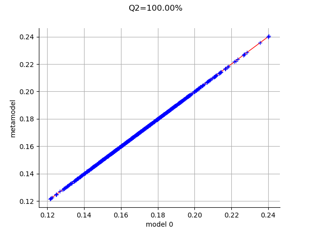
Compute the  predictivity coefficient
Q2 = val.computePredictivityFactor()[0]
Q2
Out:
0.9999977826876493
Plot the observed versus the predicted outputs.
graph = val.drawValidation()
graph.setTitle("Q2=%.2f%%" % (Q2*100))
view = viewer.View(graph)
Sensitivity analysis
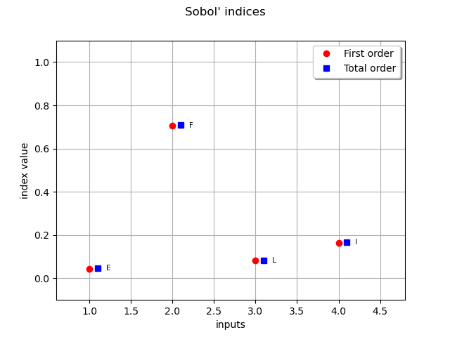
Retrieve Sobol’ sensitivity measures associated to the polynomial chaos decomposition of the model.
chaosSI = ot.FunctionalChaosSobolIndices(result)
print( chaosSI.summary() )
Out:
 input dimension: 4
 output dimension: 1
 basis size: 126
 mean: [0.170691]
 std-dev: [0.0203241]
------------------------------------------------------------
Index   | Multi-indice                  | Part of variance
------------------------------------------------------------
      2 | [0,1,0,0]                     | 0.70534
      4 | [0,0,0,1]                     | 0.164639
      3 | [0,0,1,0]                     | 0.0813041
      1 | [1,0,0,0]                     | 0.0448651
------------------------------------------------------------


------------------------------------------------------------
Component | Sobol index            | Sobol total index
------------------------------------------------------------
        0 | 0.044908               | 0.0455157
        1 | 0.70534                | 0.708258
        2 | 0.0813125              | 0.0823703
        3 | 0.165174               | 0.167125
------------------------------------------------------------
first_order = [chaosSI.getSobolIndex(i) for i in range(dim_input)]
total_order = [chaosSI.getSobolTotalIndex(i) for i in range(dim_input)]
input_names = g.getInputDescription()
graph = ot.SobolIndicesAlgorithm.DrawSobolIndices(input_names, first_order, total_order)
view = viewer.View(graph)

plt.show()
Conclusion
We see that the coefficients are particularily well computed since the Q2 coefficient is excellent (perfect ?), even with a relatively limited amount of simulation (256 points).
Total running time of the script: ( 0 minutes 0.217 seconds)