Validate a polynomial chaos

In this example, we show how to perform the draw validation of a polynomial chaos for the Ishigami function.

import openturns as ot
import openturns.viewer as viewer
from matplotlib import pylab as plt
from math import pi
ot.Log.Show(ot.Log.NONE)

Model description

We load the Ishigami test function from the usecases module :

from openturns.usecases import ishigami_function as ishigami_function
im = ishigami_function.IshigamiModel()

The IshigamiModel data class contains the input distribution in im.distributionX and the Ishigami function in im.model. We also have access to the input variable names with

input_names = im.distributionX.getDescription()

N = 100
inputTrain = im.distributionX.getSample(N)
outputTrain = im.model(inputTrain)

Create the chaos

We could use only the input and output training samples: in this case, the distribution of the input sample is computed by selecting the best distribution that fits the data.

chaosalgo = ot.FunctionalChaosAlgorithm(inputTrain, outputTrain)

Since the input distribution is known in our particular case, we instead create the multivariate basis from the distribution, that is three independent variables X1, X2 and X3.

multivariateBasis = ot.OrthogonalProductPolynomialFactory([im.X1, im.X2, im.X3])
totalDegree = 8
enumfunc = multivariateBasis.getEnumerateFunction()
P = enumfunc.getStrataCumulatedCardinal(totalDegree)
adaptiveStrategy = ot.FixedStrategy(multivariateBasis, P)

selectionAlgorithm = ot.LeastSquaresMetaModelSelectionFactory()
projectionStrategy = ot.LeastSquaresStrategy(inputTrain, outputTrain, selectionAlgorithm)

chaosalgo = ot.FunctionalChaosAlgorithm(inputTrain, outputTrain, im.distributionX, adaptiveStrategy, projectionStrategy)

chaosalgo.run()
result = chaosalgo.getResult()
metamodel = result.getMetaModel()

Validation of the metamodel

In order to validate the metamodel, we generate a test sample.

n_valid = 1000
inputTest = im.distributionX.getSample(n_valid)
outputTest = im.model(inputTest)
val = ot.MetaModelValidation(inputTest, outputTest, metamodel)
Q2 = val.computePredictivityFactor()[0]
Q2

Out:

0.9972078325177286

The Q2 is very close to 1: the metamodel is excellent.

graph = val.drawValidation()
graph.setTitle("Q2=%.2f%%" % (Q2*100))
view = viewer.View(graph)
plt.show()

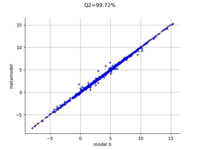
The metamodel has a good predictivity, since the points are almost on the first diagonal.