EfficientGlobalOptimization examples

The EGO algorithm (Jones, 1998) is an adaptative optimization method based on kriging.

An initial design of experiment is used to build a first metamodel. At each iteration a new point that maximizes a criterion is chosen as optimizer candidate.

The criterion uses a tradeoff between the metamodel value and the conditional variance.

Then the new point is evaluated using the original model and the metamodel is relearnt on the extended design of experiment.

import openturns as ot
import openturns.viewer as viewer
from matplotlib import pylab as plt
import math as m
ot.ResourceMap.SetAsString("KrigingAlgorithm-LinearAlgebra",  "LAPACK")
ot.Log.Show(ot.Log.NONE)

Ackley test-case

We first apply the EGO algorithm on the Ackley function.

Define the problem

The Ackley model is defined in the usecases module in a data class AckleyModel :

from openturns.usecases import ackley_function as ackley_function
am = ackley_function.AckleyModel()

We get the Ackley function :

model = am.model

We specify the domain of the model :

dim = am.dim
lowerbound = ot.Point([-4.0] * dim)
upperbound = ot.Point([4.0] * dim)

We know that the global minimum is at the center of the domain. It is stored in the AckleyModel data class.

xexact = am.x0

The minimum value attained fexact is :

fexact = model(xexact)
fexact

[4.44089e-16]

graph = model.draw(lowerbound, upperbound, [100]*dim)
graph.setTitle("Ackley function")
view = viewer.View(graph)

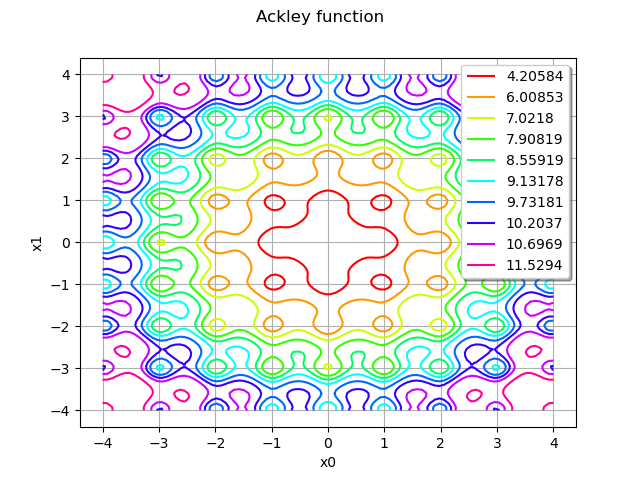
We see that the Ackley function has many local minimas. The global minimum, however, is unique and located at the center of the domain.

Create the initial kriging

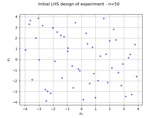
Before using the EGO algorithm, we must create an initial kriging. In order to do this, we must create a design of experiment which fills the space. In this situation, the LHSExperiment is a good place to start (but other design of experiments may allow to better fill the space). We use a uniform distribution in order to create a LHS design with 50 points.

listUniformDistributions = [ot.Uniform(lowerbound[i], upperbound[i]) for i in range(dim)]
distribution = ot.ComposedDistribution(listUniformDistributions)
sampleSize = 50
experiment = ot.LHSExperiment(distribution, sampleSize)
inputSample = experiment.generate()
outputSample = model(inputSample)

graph = ot.Graph("Initial LHS design of experiment - n=%d" % (sampleSize), "$x_0$", "$x_1$", True)
cloud = ot.Cloud(inputSample)
graph.add(cloud)
view = viewer.View(graph)

We now create the kriging metamodel. We selected the SquaredExponential covariance model with a constant basis (the MaternModel may perform better in this case). We use default settings (1.0) for the scale parameters of the covariance model, but configure the amplitude to 0.1, which better corresponds to the properties of the Ackley function.

covarianceModel = ot.SquaredExponential([1.0] * dim, [0.5])
basis = ot.ConstantBasisFactory(dim).build()
kriging = ot.KrigingAlgorithm(inputSample, outputSample, covarianceModel, basis)
kriging.run()

Create the optimization problem

We finally create the OptimizationProblem and solve it with EfficientGlobalOptimization.

problem = ot.OptimizationProblem()
problem.setObjective(model)
bounds = ot.Interval(lowerbound, upperbound)
problem.setBounds(bounds)

In order to show the various options, we configure them all, even if most could be left to default settings in this case.

The most important method is setMaximumEvaluationNumber which limits the number of iterations that the algorithm can perform. In the Ackley example, we choose to perform 10 iterations of the algorithm.

algo = ot.EfficientGlobalOptimization(problem, kriging.getResult())
algo.setMaximumEvaluationNumber(10)
algo.run()
result = algo.getResult()

result.getIterationNumber()

Out:

10

result.getOptimalPoint()

[0.0782936,0.0108398]

result.getOptimalValue()

[0.381764]

fexact

[4.44089e-16]

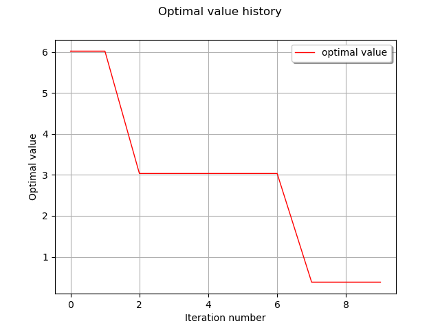
Compared to the minimum function value, we see that the EGO algorithm provides solution which is not very accurate. However, the optimal point is in the neighbourhood of the exact solution, and this is quite an impressive success given the limited amount of function evaluations: only 60 evaluations for the initial DOE and 10 iterations of the EGO algorithm, for a total equal to 70 function evaluations.

graph = result.drawOptimalValueHistory()
view = viewer.View(graph)

inputHistory = result.getInputSample()

graph = model.draw(lowerbound, upperbound, [100]*dim)
graph.setLegends([""])
graph.setTitle("Ackley function. Initial : black bullet. Solution : green diamond.")
cloud = ot.Cloud(inputSample)
cloud.setPointStyle("bullet")
cloud.setColor("black")
graph.add(cloud)
cloud = ot.Cloud(inputHistory)
cloud.setPointStyle("diamond")
cloud.setColor("forestgreen")
graph.add(cloud)
view = viewer.View(graph)

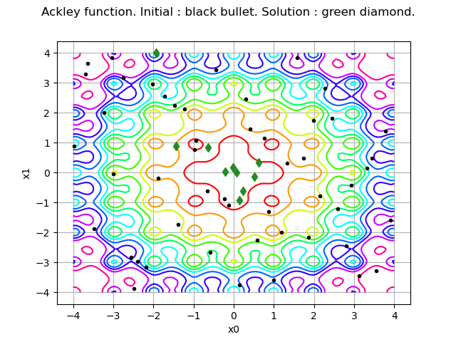
We see that the initial (black) points are dispersed in the whole domain, while the solution points are much closer to the solution.

However, the final solution produced by the EGO algorithm is not very accurate. This is why we finalize the process by adding a local optimization step.

algo2 = ot.NLopt(problem, 'LD_LBFGS')
algo2.setStartingPoint(result.getOptimalPoint())
algo2.run()
result = algo2.getResult()

result.getOptimalPoint()

[1.48118e-08,-9.31735e-09]

The corrected solution is now extremely accurate.

graph = result.drawOptimalValueHistory()
view = viewer.View(graph)

Branin test-case

We now take a look at the Branin-Hoo function.

Define the problem

The Branin model is defined in the usecases module in a data class BraninModel :

from openturns.usecases import branin_function as branin_function
bm = branin_function.BraninModel()

We load the dimension,

dim = bm.dim

the domain boundaries,

lowerbound = bm.lowerbound
upperbound = bm.upperbound

and we load the model function :

model = bm.model
objectiveFunction = model.getMarginal(0)

We build a sample out of the three minima :

xexact = ot.Sample([bm.xexact1, bm.xexact2, bm.xexact3])

The minimum value attained fexact is :

fexact = objectiveFunction(xexact)
fexact

	y0
0	-0.9794764
1	-0.9794764
2	-0.9794764

graph = objectiveFunction.draw(lowerbound, upperbound, [100]*dim)
graph.setTitle("Branin function")
view = viewer.View(graph)

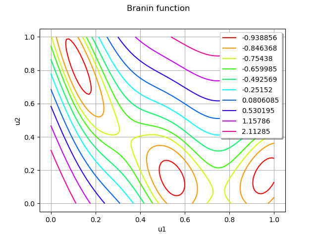
The Branin function has three local minimas.

Create the initial kriging

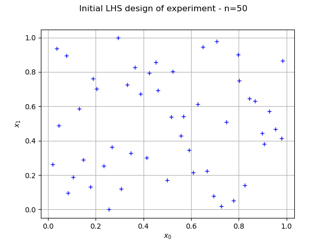
distribution = ot.ComposedDistribution([ot.Uniform(0.0, 1.0)] * dim)
sampleSize = 50
experiment = ot.LHSExperiment(distribution, sampleSize)
inputSample = experiment.generate()
modelEval = model(inputSample)
outputSample = modelEval.getMarginal(0)

graph = ot.Graph("Initial LHS design of experiment - n=%d" % (sampleSize), "$x_0$", "$x_1$", True)
cloud = ot.Cloud(inputSample)
graph.add(cloud)
view = viewer.View(graph)

covarianceModel = ot.SquaredExponential([1.0] * dim, [1.0])
basis = ot.ConstantBasisFactory(dim).build()
kriging = ot.KrigingAlgorithm(inputSample, outputSample, covarianceModel, basis)

noise = [x[1] for x in modelEval]
kriging.setNoise(noise)
kriging.run()

Create and solve the problem

We define the problem :

problem = ot.OptimizationProblem()
problem.setObjective(model)
bounds = ot.Interval(lowerbound, upperbound)
problem.setBounds(bounds)

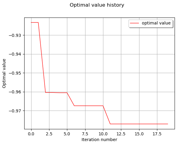
We configure the maximum number of function evaluations to 20. We assume that the function is noisy, with a constant variance.

We configure the algorithm :

algo = ot.EfficientGlobalOptimization(problem, kriging.getResult())
# assume constant noise var
guessedNoiseFunction = 0.1
noiseModel = ot.SymbolicFunction(['x1', 'x2'], [str(guessedNoiseFunction)])
algo.setNoiseModel(noiseModel)
algo.setMaximumEvaluationNumber(20)
algo.run()
result = algo.getResult()

result.getIterationNumber()

Out:

20

result.getOptimalPoint()

[0.529867,0.154731]

result.getOptimalValue()

[-0.977061]

fexact

	y0
0	-0.9794764
1	-0.9794764
2	-0.9794764

inputHistory = result.getInputSample()

graph = objectiveFunction.draw(lowerbound, upperbound, [100]*dim)
graph.setLegends([""])
graph.setTitle("Branin function. Initial : black bullet. Solution : green diamond.")
cloud = ot.Cloud(inputSample)
cloud.setPointStyle("bullet")
cloud.setColor("black")
graph.add(cloud)
cloud = ot.Cloud(inputHistory)
cloud.setPointStyle("diamond")
cloud.setColor("forestgreen")
graph.add(cloud)
view = viewer.View(graph)

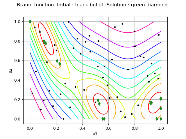
We see that the EGO algorithm found the second local minimum. Given the limited number of function evaluations, the other local minimas have not been explored.

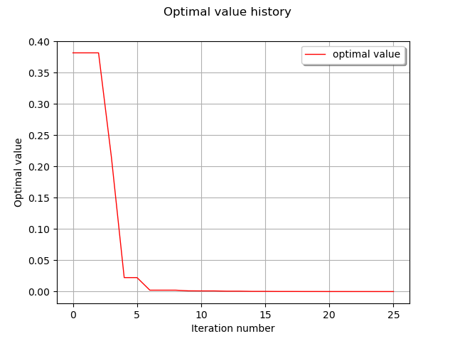
graph = result.drawOptimalValueHistory()
view = viewer.View(graph)

plt.show()