Distribution manipulation

In this example we are going to exhibit some of the services exposed by the distribution objects:

• ask for the dimension, with the method getDimension

• extract the marginal distributions, with the method getMarginal

• to ask for some properties, with isContinuous, isDiscrete, isElliptical

• to get the copula, with the method getCopula*

• to ask for some properties on the copula, with the methods hasIndependentCopula, hasEllipticalCopula

• to evaluate some moments, with getMean, getStandardDeviation, getCovariance, getSkewness, getKurtosis

• to evaluate the roughness, with the method getRoughness

• to get one realization or simultaneously realizations, with the method getRealization, getSample

• to evaluate the probability content of a given interval, with the method computeProbability

• to evaluate a quantile or a complementary quantile, with the method computeQuantile

• to evaluate the characteristic function of the distribution

• to evaluate the derivative of the CDF or PDF

• to draw some curves

from __future__ import print_function
import openturns as ot
import openturns.viewer as viewer
from matplotlib import pylab as plt
ot.Log.Show(ot.Log.NONE)

Create an 1-d distribution

dist_1 = ot.Normal()

# Create a 2-d distribution
dist_2 = ot.ComposedDistribution([ot.Normal(), ot.Triangular(0.0, 2.0, 3.0)], ot.ClaytonCopula(2.3))

# Create a 3-d distribution
copula_dim3 = ot.Student(5.0, 3).getCopula()
dist_3 = ot.ComposedDistribution([ot.Normal(), ot.Triangular(0.0, 2.0, 3.0), ot.Exponential(0.2)], copula_dim3)

Get the dimension fo the distribution

dist_2.getDimension()

Out:

2

Get the 2nd marginal

dist_2.getMarginal(1)

Triangular(a = 0, m = 2, b = 3)

Get a 2-d marginal

dist_3.getMarginal([0, 1]).getDimension()

Out:

2

Ask some properties of the distribution

dist_1.isContinuous(), dist_1.isDiscrete(), dist_1.isElliptical()

Out:

(True, False, True)

Get the copula

copula = dist_2.getCopula()

Ask some properties on the copula

dist_2.hasIndependentCopula(), dist_2.hasEllipticalCopula()

Out:

(False, False)

mean vector of the distribution

dist_2.getMean()

[0,1.66667]

standard deviation vector of the distribution

dist_2.getStandardDeviation()

[1,0.62361]

covariance matrix of the distribution

dist_2.getCovariance()

[[ 1 0.491927 ]
[ 0.491927 0.388889 ]]

skewness vector of the distribution

dist_2.getSkewness()

[0,-0.305441]

kurtosis vector of the distribution

dist_2.getKurtosis()

[3,2.4]

roughness of the distribution

dist_1.getRoughness()

Out:

0.28209479177387814

Get one realization

dist_2.getRealization()

[0.779052,2.64799]

Get several realizations

dist_2.getSample(5)

	X0	X1
0	0.06985929	1.42593
1	-0.2847443	1.680554
2	-1.842467	0.7630956
3	0.3236553	2.048827
4	0.1203091	2.285018

Evaluate the PDF at the mean point

dist_2.computePDF(dist_2.getMean())

Out:

0.3528005531670077

Evaluate the CDF at the mean point

dist_2.computeCDF(dist_2.getMean())

Out:

0.3706626446357781

Evaluate the complementary CDF

dist_2.computeComplementaryCDF(dist_2.getMean())

Out:

0.6293373553642219

Evaluate the survival function at the mean point

dist_2.computeSurvivalFunction(dist_2.getMean())

Out:

0.4076996816728151

Evaluate the PDF on a sample

dist_2.computePDF(dist_2.getSample(5))

	v0
0	0.2107205
1	0.2829345
2	0.2683372
3	0.3159856
4	0.3618715

Evaluate the CDF on a sample

dist_2.computeCDF(dist_2.getSample(5))

	v0
0	0.7326854
1	0.5003563
2	0.820944
3	0.01091264
4	0.4877803

Evaluate the probability content of an 1-d interval

interval = ot.Interval(-2.0, 3.0)
dist_1.computeProbability(interval)

Out:

0.9758999700201907

Evaluate the probability content of a 2-d interval

interval = ot.Interval([0.4, -1], [3.4, 2])
dist_2.computeProbability(interval)

Out:

0.129833882783416

Evaluate the quantile of order p=90%

dist_2.computeQuantile(0.90)

[1.60422,2.59627]

and the quantile of order 1-p

dist_2.computeQuantile(0.90, True)

[-1.10363,0.899591]

Evaluate the quantiles of order p et q For example, the quantile 90% and 95%

dist_1.computeQuantile([0.90, 0.95])

	v0
0	1.281552
1	1.644854

and the quantile of order 1-p and 1-q

dist_1.computeQuantile([0.90, 0.95], True)

	v0
0	-1.281552
1	-1.644854

Evaluate the characteristic function of the distribution (only 1-d)

dist_1.computeCharacteristicFunction(dist_1.getMean()[0])

Out:

(1+0j)

Evaluate the derivatives of the PDF with respect to the parameters at mean

dist_2.computePDFGradient(dist_2.getMean())

[0,-0.398942,0.12963,-0.277778,-0.185185,0]

Evaluate the derivatives of the CDF with respect to the parameters at mean

dist_2.computeCDFGradient(dist_2.getMean())

[-0.398942,-0,-0.169753,-0.231481,-0.555556,0]

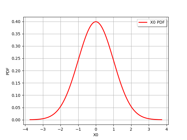
draw PDF

graph = dist_1.drawPDF()
view = viewer.View(graph)

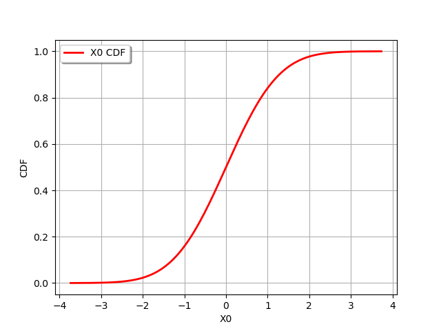
draw CDF

graph = dist_1.drawCDF()
view = viewer.View(graph)

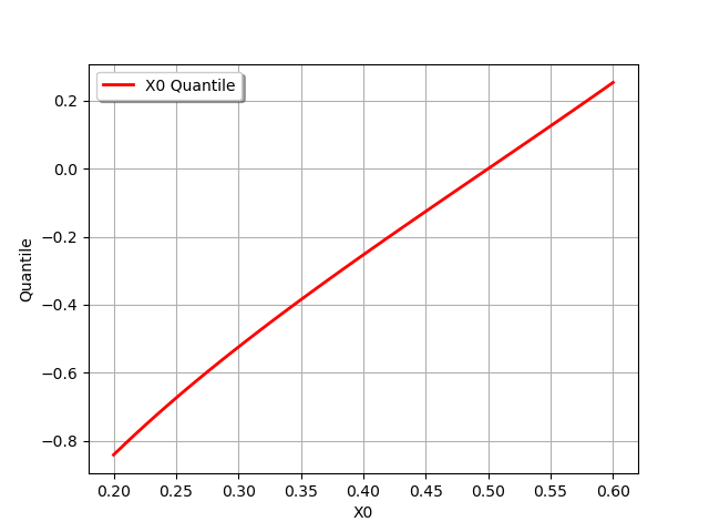
Draw an 1-d quantile curve

# Define the range and the number of points
qMin = 0.2
qMax = 0.6
nbrPoints = 101
quantileGraph = dist_1.drawQuantile(qMin, qMax, nbrPoints)
view = viewer.View(quantileGraph)

Draw a 2-d quantile curve

# Define the range and the number of points
qMin = 0.3
qMax = 0.9
nbrPoints = 101
quantileGraph = dist_2.drawQuantile(qMin, qMax, nbrPoints)
view = viewer.View(quantileGraph)
plt.show()