Draw minimum volume level set in 2D

In this example, we compute the minimum volume level set of a bivariate distribution.

import openturns as ot
import openturns.viewer as viewer
from matplotlib import pylab as plt
ot.Log.Show(ot.Log.NONE)

Create a gaussian

corr = ot.CorrelationMatrix(2)
corr[0, 1] = 0.2
copula = ot.NormalCopula(corr)
x1 = ot.Normal(-1., 1)
x2 = ot.Normal(2, 1)
x_funk = ot.ComposedDistribution([x1, x2], copula)

# Create a second gaussian
x1 = ot.Normal(1.,1)
x2 = ot.Normal(-2,1)
x_punk = ot.ComposedDistribution([x1, x2], copula)

# Mix the distributions
mixture = ot.Mixture([x_funk, x_punk], [0.5,1.])

graph = mixture.drawPDF()
view = viewer.View(graph)

For a multivariate distribution (with dimension greater than 1), the computeMinimumVolumeLevelSetWithThreshold uses Monte-Carlo sampling.

ot.ResourceMap.SetAsUnsignedInteger("Distribution-MinimumVolumeLevelSetSamplingSize",1000)

We want to compute the minimum volume LevelSet which contains alpha`=90% of the distribution. The `threshold is the value of the PDF corresponding the alpha-probability: the points contained in the LevelSet have a PDF value lower or equal to this threshold.

alpha = 0.9
levelSet, threshold = mixture.computeMinimumVolumeLevelSetWithThreshold(alpha)
threshold

Out:

0.009132175837384555

def drawLevelSetContour2D(distribution, numberOfPointsInXAxis, alpha, threshold, sampleSize= 500):
    '''
    Compute the minimum volume LevelSet of measure equal to alpha and get the
    corresponding density value (named threshold).
    Generate a sample of the distribution and draw it.
    Draw a contour plot for the distribution, where the PDF is equal to threshold.
    '''
    sample = distribution.getSample(sampleSize)
    X1min = sample[:, 0].getMin()[0]
    X1max = sample[:, 0].getMax()[0]
    X2min = sample[:, 1].getMin()[0]
    X2max = sample[:, 1].getMax()[0]
    xx = ot.Box([numberOfPointsInXAxis],
                ot.Interval([X1min], [X1max])).generate()
    yy = ot.Box([numberOfPointsInXAxis],
                ot.Interval([X2min], [X2max])).generate()
    xy = ot.Box([numberOfPointsInXAxis, numberOfPointsInXAxis],
                ot.Interval([X1min, X2min], [X1max, X2max])).generate()
    data = distribution.computePDF(xy)
    graph = ot.Graph('', 'X1', 'X2', True, 'topright')
    labels = ["%.2f%%" % (100*alpha)]
    contour = ot.Contour(xx, yy, data, ot.Point([threshold]), ot.Description(labels))
    contour.setColor('black')
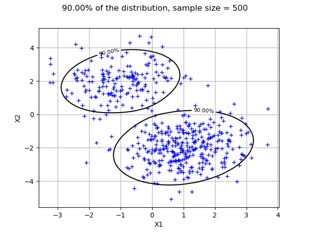
    graph.setTitle("%.2f%% of the distribution, sample size = %d" % (100*alpha,sampleSize))
    graph.add(contour)
    cloud = ot.Cloud(sample)
    graph.add(cloud)
    return graph

The following plot shows that 90% of the sample is contained in the LevelSet.

numberOfPointsInXAxis = 50
graph = drawLevelSetContour2D(mixture, numberOfPointsInXAxis, alpha, threshold)
view = viewer.View(graph)
plt.show()