ARMA process manipulation

In this example we will expose some of the services exposed by an object, namely:

• its AR and MA coefficients thanks to the methods getARCoefficients, getMACoefficients,

• its white noise thanks to the method getWhiteNoise, that contains the time grid of the process,

• its current state, that is its last values and the last values of its white noise, thanks to the method getState,

• a realization thanks to the method getRealization or a sample of realizations thanks to the method getSample,

• a possible future of the model, which is a possible prolongation of the current state on the next instants, thanks to the method getFuture.

• possible futures of the model, which correspond to possible prolongations of the current state on the next instants, thanks to the method getFuture (, ).

from __future__ import print_function
import openturns as ot
import openturns.viewer as viewer
from matplotlib import pylab as plt
import math as m
ot.Log.Show(ot.Log.NONE)

Create an ARMA process

# Create the mesh
tMin = 0.
time_step = 0.1
n = 100
time_grid = ot.RegularGrid(tMin, time_step, n)

# Create the distribution of dimension 1 or 3
# Care : the mean must be NULL
myDist_1 = ot.Triangular(-1., 0.0, 1.)

# Create  a white noise of dimension 1
myWN_1d = ot.WhiteNoise(myDist_1, time_grid)

# Create the ARMA model : ARMA(4,2) in dimension 1
myARCoef = ot.ARMACoefficients([0.4, 0.3, 0.2, 0.1])
myMACoef = ot.ARMACoefficients([0.4, 0.3])
arma = ot.ARMA(myARCoef, myMACoef, myWN_1d)

Check the linear recurrence

arma

ARMA(X_{0,t} + 0.4 X_{0,t-1} + 0.3 X_{0,t-2} + 0.2 X_{0,t-3} + 0.1 X_{0,t-4} = E_{0,t} + 0.4 E_{0,t-1} + 0.3 E_{0,t-2}, E_t ~ Triangular(a = -1, m = 0, b = 1))

Get the coefficients of the recurrence

print('AR coeff = ', arma.getARCoefficients())
print('MA coeff = ', arma.getMACoefficients())

Out:

AR coeff =  shift = 0
[[ 0.4 ]]
shift = 1
[[ 0.3 ]]
shift = 2
[[ 0.2 ]]
shift = 3
[[ 0.1 ]]

MA coeff =  shift = 0
[[ 0.4 ]]
shift = 1
[[ 0.3 ]]

Get the white noise

myWhiteNoise = arma.getWhiteNoise()
myWhiteNoise

WhiteNoise(Triangular(a = -1, m = 0, b = 1))

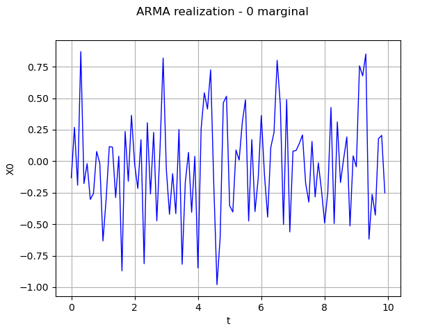
Generate one time series

ts = arma.getRealization()
ts.setName('ARMA realization')

Draw the time series : marginal index 0

graph = ts.drawMarginal(0)
view = viewer.View(graph)

Generate a k time series

k = 5
myProcessSample = arma.getSample(k)

# Then get the current state of the ARMA
armaState = arma.getState()
# From the armaState, get the last values
myLastValues = armaState.getX()
# From the ARMAState, get the last noise values
myLastEpsilonValues = armaState.getEpsilon()

Get the number of iterations before getting a stationary state

arma.getNThermalization()

Out:

75

This may be important to evaluate it with another precision epsilon

epsilon = 1e-8
newThermalValue = arma.computeNThermalization(epsilon)
arma.setNThermalization(newThermalValue)

Make a prediction from the curent state of the ARMA on the next Nit instants

Nit = 100
# at first, specify a current state armaState
arma = ot.ARMA(myARCoef, myMACoef, myWhiteNoise, armaState)

# then, generate a possible future
future = arma.getFuture(Nit)

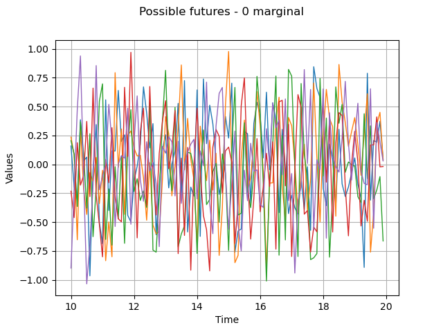
Generate N possible futures on the Nit next points

N = 5
possibleFuture_N = arma.getFuture(Nit, N)
possibleFuture_N.setName('Possible futures')

# Draw the future : marginal index 0
graph = possibleFuture_N.drawMarginal(0)
view = viewer.View(graph)
plt.show()