Process manipulation

The objective here is to manipulate a multivariate stochastic process , where is discretized on the mesh and exhibit some of the services exposed by the Process objects:

• ask for the dimension, with the method getOutputDimension

• ask for the mesh, with the method getMesh

• ask for the mesh as regular 1-d mesh, with the getTimeGrid method

• ask for a realization, with the method the getRealization method

• ask for a continuous realization, with the getContinuousRealization method

• ask for a sample of realizations, with the getSample method

• ask for the normality of the process with the isNormal method

• ask for the stationarity of the process with the isStationary method

from __future__ import print_function
import openturns as ot
import openturns.viewer as viewer
from matplotlib import pylab as plt
import math as m
ot.Log.Show(ot.Log.NONE)

Create a mesh which is a RegularGrid

tMin = 0.0
timeStep = 0.1
n = 100
time_grid = ot.RegularGrid(tMin, timeStep, n)
time_grid.setName('time')

Create a process of dimension 3 Normal process with an Exponential covariance model Amplitude and scale values of the Exponential model

scale = [4.0]
amplitude = [1.0, 2.0, 3.0]
# spatialCorrelation
spatialCorrelation = ot.CorrelationMatrix(3)
spatialCorrelation[0, 1] = 0.8
spatialCorrelation[0, 2] = 0.6
spatialCorrelation[1, 2] = 0.1
myCovarianceModel = ot.ExponentialModel(scale, amplitude, spatialCorrelation)
process = ot.GaussianProcess(myCovarianceModel, time_grid)

Get the dimension d of the process

process.getOutputDimension()

Out:

3

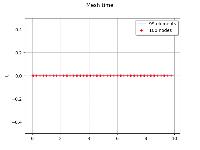
Get the mesh of the process

mesh = process.getMesh()

# Get the corners of the mesh
minMesh = mesh.getVertices().getMin()[0]
maxMesh = mesh.getVertices().getMax()[0]
graph = mesh.draw()
view = viewer.View(graph)

Get the time grid of the process only when the mesh can be interpreted as a regular time grid

process.getTimeGrid()

RegularGrid(start=0, step=0.1, n=100)

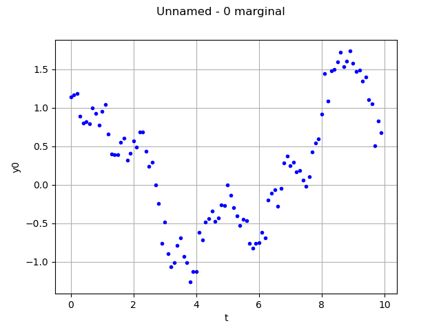
Get a realisation of the process

realization = process.getRealization()
#realization

Draw one realization

interpolate=False
graph = realization.drawMarginal(0, interpolate)
view = viewer.View(graph)

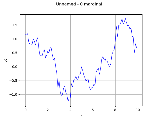
Same graph, but draw interpolated values

graph = realization.drawMarginal(0)
view = viewer.View(graph)

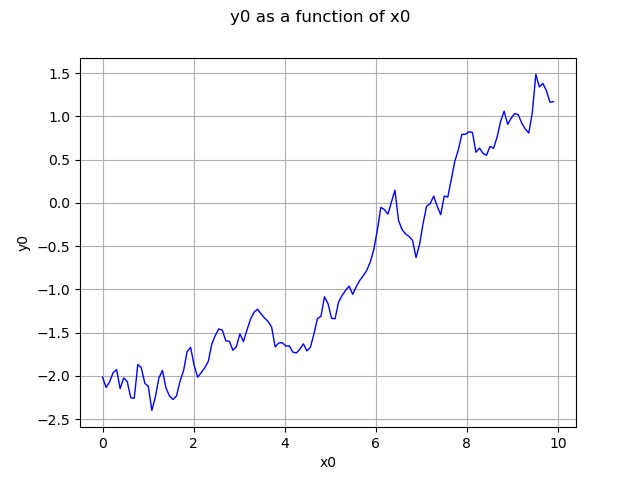
Get a function representing the process using P1 Lagrange interpolation (when not defined from a functional model)

continuousRealization = process.getContinuousRealization()

Draw its first marginal

marginal0 = continuousRealization.getMarginal(0)
graph = marginal0.draw(minMesh, maxMesh)
view = viewer.View(graph)

Get several realizations of the process

number = 10
fieldSample = process.getSample(number)
#fieldSample

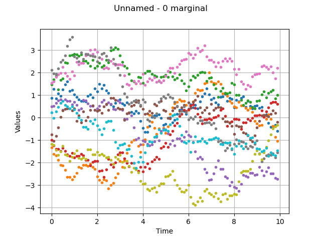
Draw a sample of the process

graph = fieldSample.drawMarginal(0, False)
view = viewer.View(graph)

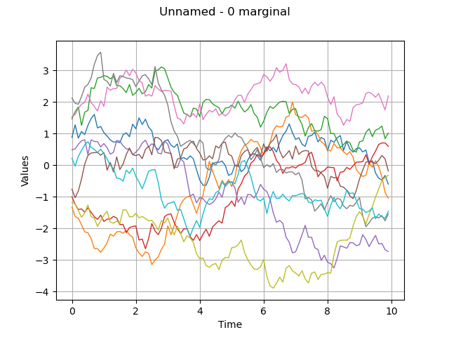
Same graph, but draw interpolated values

graph = fieldSample.drawMarginal(0)
view = viewer.View(graph)

Get the marginal of the process at index 1 Care! Numerotation begins at 0 Not yet implemented for some processes

process.getMarginal([1])

GaussianProcess(trend=[x0]->[0.0], covariance=ExponentialModel(scale=[4], amplitude=[2], no spatial correlation))

Get the marginal of the process at index in indices Not yet implemented for some processes

process.getMarginal([0, 1])

GaussianProcess(trend=[x0]->[0.0,0.0], covariance=ExponentialModel(scale=[4], amplitude=[1,2], spatial correlation=
[[ 1 0.8 ]
[ 0.8 1 ]]))

Check wether the process is normal

process.isNormal()

Out:

True

Check wether the process is stationary

process.isStationary()

plt.show()