Create a design of experiments with discrete and continuous variables

In this example we present how to create a design of experiments when one (or several) of the marginals are discrete.

from __future__ import print_function
import openturns as ot
import openturns.viewer as viewer
from matplotlib import pylab as plt
ot.Log.Show(ot.Log.NONE)

To create the first marginal of the distribution, we select a univariate discrete distribution. Some of them, like the Bernoulli or Geometric distributions, are implemented in the library as classes. In this example however, we pick the UserDefined distribution that assigns equal weights to the values -2, -1, 1 and 2.

sample = ot.Sample([[-2.], [-1.], [1.], [2.]])
sample

	v0
0	-2
1	-1
2	1
3	2

X0 = ot.UserDefined(sample)

For the second marginal, we pick a Gaussian distribution.

X1 = ot.Normal()

Create the multivariate distribution from its marginals and an independent copula.

distribution = ot.ComposedDistribution([X0,X1])

Create the design.

size = 100
experiment = ot.MonteCarloExperiment(distribution, size)
sample = experiment.generate()

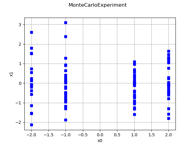
Plot the design.

graph = ot.Graph("MonteCarloExperiment", "x0", "x1", True, "")
cloud = ot.Cloud(sample, "blue", "fsquare", "")
graph.add(cloud)
view = viewer.View(graph)

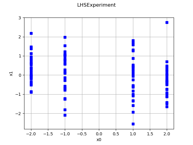
Any other type of design of experiments can be generated based on this distribution. The following example shows a LHS experiment.

size = 100
alwaysShuffle = True
randomShift = True
experiment = ot.LHSExperiment(distribution, size, alwaysShuffle, randomShift)
sample = experiment.generate()

graph = ot.Graph("LHSExperiment", "x0", "x1", True, "")
cloud = ot.Cloud(sample, "blue", "fsquare", "")
graph.add(cloud)
view = viewer.View(graph)
plt.show()