Various design of experiments in OpenTURNS

The goal of this example is to present several design of experiments available in OpenTURNS.

Distribution

import openturns as ot
import openturns.viewer as otv
import pylab as pl
import openturns.viewer as viewer
from matplotlib import pylab as plt
ot.Log.Show(ot.Log.NONE)

Monte-Carlo sampling in 2D

dim = 2
X = [ot.Uniform()] * dim
distribution = ot.ComposedDistribution(X)
bounds = distribution.getRange()

sampleSize = 10
sample = distribution.getSample(sampleSize)

fig = otv.PlotDesign(sample, bounds);

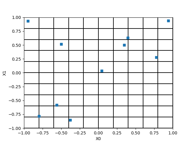
We see that there a empty zones in the input space.

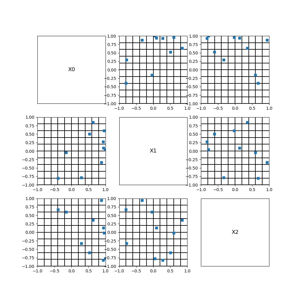
Monte-Carlo sampling in 3D

dim = 3
X = [ot.Uniform()] * dim
distribution = ot.ComposedDistribution(X)
bounds = distribution.getRange()

sampleSize = 10
sample = distribution.getSample(sampleSize)

fig = otv.PlotDesign(sample, bounds)
fig.set_size_inches(10, 10)

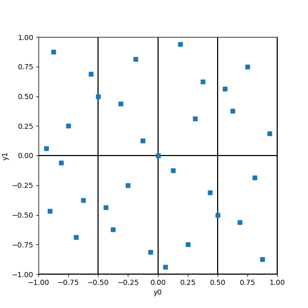
Latin Hypercube Sampling

distribution = ot.ComposedDistribution([ot.Uniform()]*3)
samplesize = 5
experiment = ot.LHSExperiment(distribution, samplesize, False, False)
sample = experiment.generate()

In order to see the LHS property, we need to set the bounds.

bounds = distribution.getRange()

fig = otv.PlotDesign(sample, bounds)
fig.set_size_inches(10, 10)

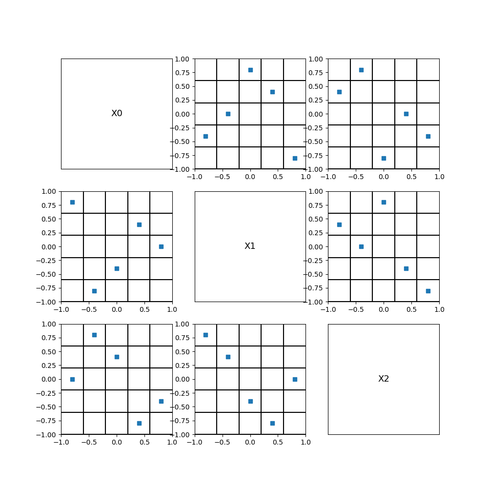
We see that each column or row exactly contains one single point. This shows that a LHS design of experimens has good 1D projection properties, and, hence, is a good candidate for a space filling design.

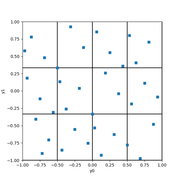
Optimized LHS

distribution = ot.ComposedDistribution([ot.Uniform()]*3)
samplesize = 10

bounds = distribution.getRange()

lhs = ot.LHSExperiment(distribution, samplesize)
lhs.setAlwaysShuffle(True) # randomized
space_filling = ot.SpaceFillingC2()
temperatureProfile = ot.GeometricProfile(10.0, 0.95, 1000)
algo = ot.SimulatedAnnealingLHS(lhs, temperatureProfile, space_filling)
# optimal design
sample = algo.generate()

fig = otv.PlotDesign(sample, bounds)
fig.set_size_inches(10, 10)

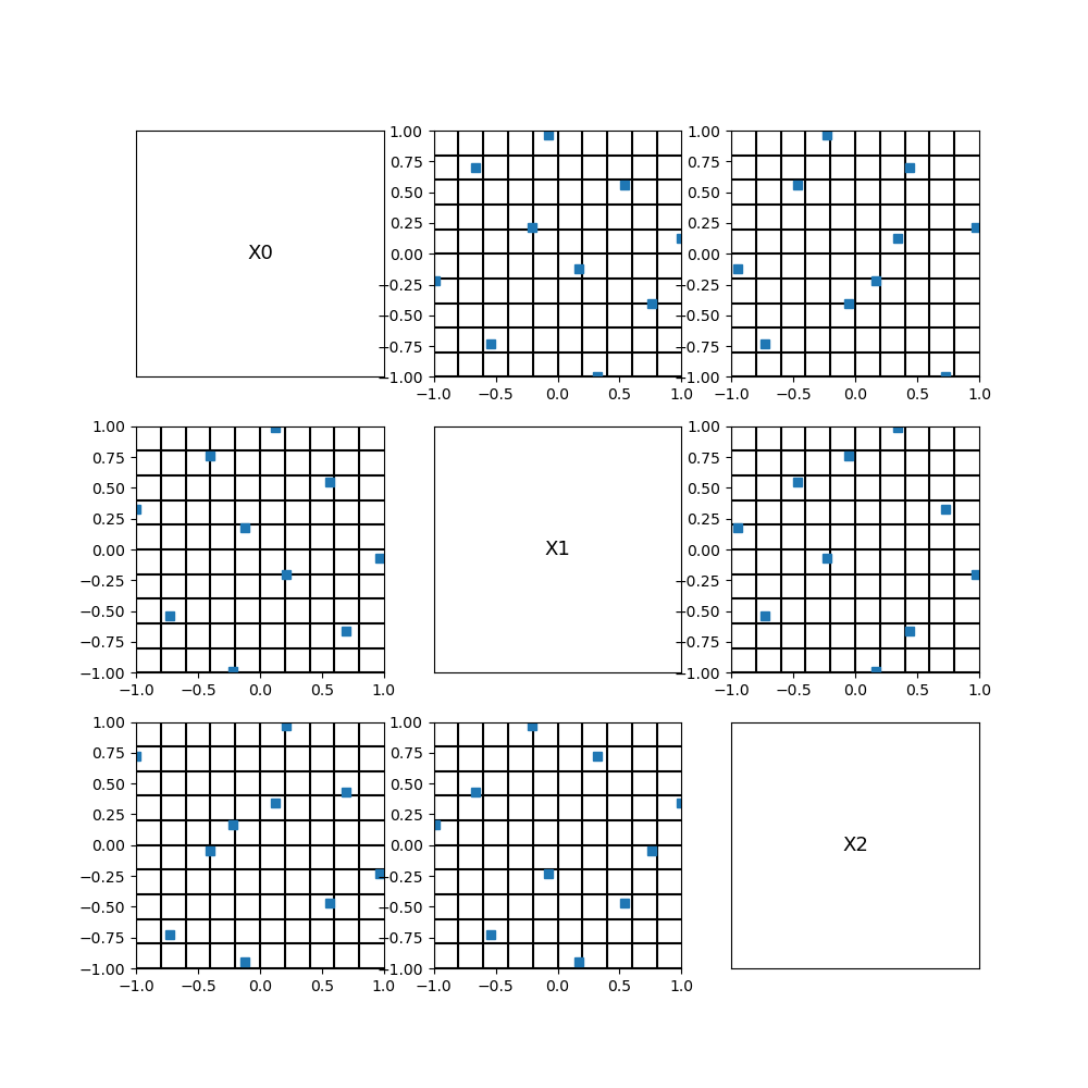
We see that this LHS is optimized in the sense that it fills the space more evenly than a non-optimized does in general.

Sobol’ low discrepancy sequence

dim = 2
distribution = ot.ComposedDistribution([ot.Uniform()]*dim)
bounds = distribution.getRange()

sequence = ot.SobolSequence(dim)

samplesize = 2**5 # Sobol' sequences are in base 2
experiment = ot.LowDiscrepancyExperiment(sequence, distribution, samplesize, False)
sample = experiment.generate()

samplesize

Out:

32

subdivisions = [2**2, 2**1]
fig = otv.PlotDesign(sample, bounds, subdivisions);
fig.set_size_inches(6, 6)

We have elementary intervals in 2 dimensions, each having a volume equal to 1/8. Since there are 32 points, the Sobol’ sequence is so that each elementary interval contains exactly 32/8 = 4 points. Notice that each elementary interval is closed on the left (or bottom) and open on the right (or top).

Halton low discrepancy sequence

dim = 2
distribution = ot.ComposedDistribution([ot.Uniform()]*dim)
bounds = distribution.getRange()

sequence = ot.HaltonSequence(dim)

samplesize = 2**2 * 3**2 # Halton sequence uses prime numbers 2 and 3 in two dimensions.
experiment = ot.LowDiscrepancyExperiment(sequence, distribution, samplesize, False)
sample = experiment.generate()

samplesize

Out:

36

subdivisions = [2**2, 3]
fig = otv.PlotDesign(sample, bounds, subdivisions);
fig.set_size_inches(6, 6)

We have elementary intervals in 2 dimensions, each having a volume equal to 1/12. Since there are 36 points, the Halton sequence is so that each elementary interval contains exactly 36/12 = 3 points. Notice that each elementary interval is closed on the left (or bottom) and open on the right (or top).