Create and draw scalar distributions

from __future__ import print_function
import openturns as ot
import openturns.viewer as viewer
from matplotlib import pylab as plt
ot.Log.Show(ot.Log.NONE)

A continuous distribution

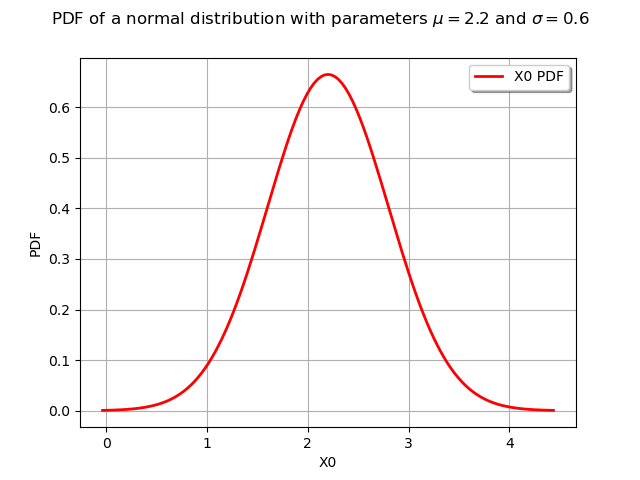
We build a normal distribution with parameters :

distribution = ot.Normal(2.2, 0.6)
print(distribution)

Out:

Normal(mu = 2.2, sigma = 0.6)

We can draw a sample following this distribution with the getSample method :

size = 10
sample = distribution.getSample(size)
print(sample)

Out:

    [ X0      ]
0 : [ 2.90698 ]
1 : [ 2.4694  ]
2 : [ 2.37417 ]
3 : [ 2.69831 ]
4 : [ 2.28606 ]
5 : [ 2.08412 ]
6 : [ 2.87742 ]
7 : [ 1.80004 ]
8 : [ 1.67943 ]
9 : [ 2.99115 ]

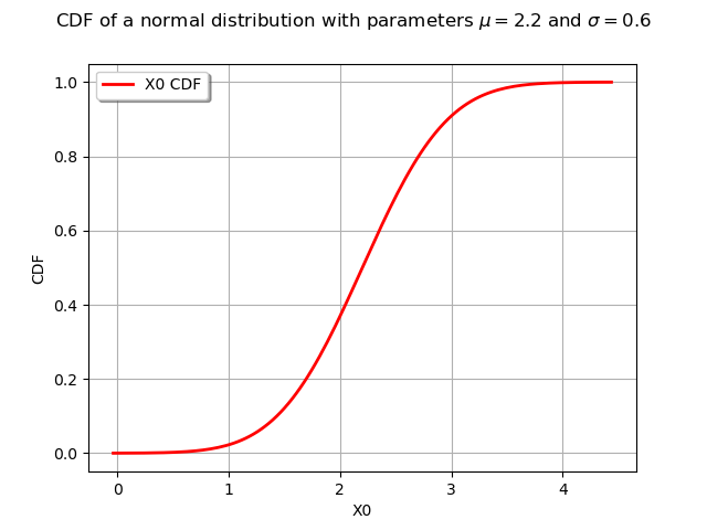
We draw its PDF and CDF :

graphPDF = distribution.drawPDF()
graphPDF.setTitle(r"PDF of a normal distribution with parameters $\mu = 2.2$ and $\sigma = 0.6$")
view = viewer.View(graphPDF)

graphCDF = distribution.drawCDF()
graphCDF.setTitle(r"CDF of a normal distribution with parameters $\mu = 2.2$ and $\sigma = 0.6$")
view = viewer.View(graphCDF)

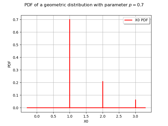
A discrete distribution

We define a geometric distribution with parameter .

p = 0.7
distribution = ot.Geometric(p)
print(distribution)

Out:

Geometric(p = 0.7)

We draw a sample of it :

size = 10
sample = distribution.getSample(size)
print(sample)

Out:

    [ X0 ]
0 : [ 3  ]
1 : [ 1  ]
2 : [ 1  ]
3 : [ 2  ]
4 : [ 1  ]
5 : [ 2  ]
6 : [ 1  ]
7 : [ 1  ]
8 : [ 1  ]
9 : [ 2  ]

We draw its PDF and its CDF :

graphPDF = distribution.drawPDF()
graphPDF.setTitle(r"PDF of a geometric distribution with parameter $p = 0.7$")
view = viewer.View(graphPDF)

graphCDF = distribution.drawCDF()
graphCDF.setTitle(r"CDF of a geometric distribution with parameter $p = 0.7$")
view = viewer.View(graphCDF)

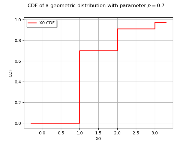
Conclusion

The two previous examples look very similar despite their continuous and discrete nature. In the library there is no distinction between continuous and discrete distributions.

Display all figures

plt.show()