Transform a distribution

In this example we are going to use distribution algebra and distribution transformation via functions.

from __future__ import print_function
import openturns as ot
import openturns.viewer as viewer
from matplotlib import pylab as plt
ot.Log.Show(ot.Log.NONE)

We define some (classical) distributions :

distribution1 = ot.Uniform(0.0, 1.0)
distribution2 = ot.Uniform(0.0, 2.0)
distribution3 = ot.WeibullMin(1.5, 2.0)

Sum & difference of distributions

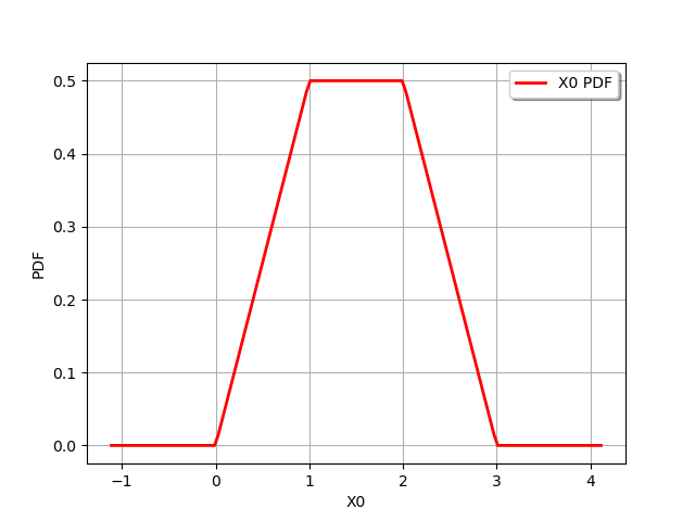
It is easy to compute the sum of distributions. For example :

distribution = distribution1 + distribution2
print(distribution)
graph = distribution.drawPDF()
view = viewer.View(graph)

Out:

Trapezoidal(a = 0, b = 1, c = 2, d = 3)

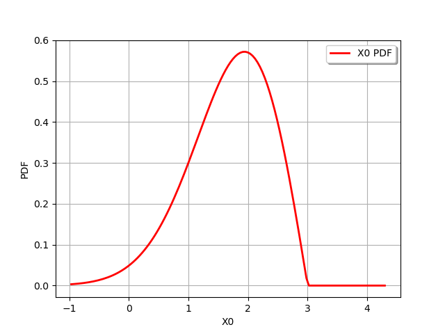
We might also use substraction even with scalar values :

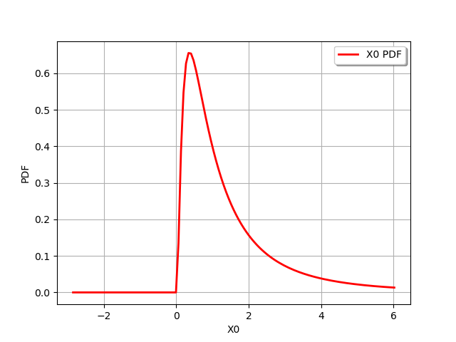
distribution = 3.0 - distribution3
print(distribution)
graph = distribution.drawPDF()
view = viewer.View(graph)

Out:

RandomMixture(3 - WeibullMin(beta = 1.5, alpha = 2, gamma = 0))

Product & inverse

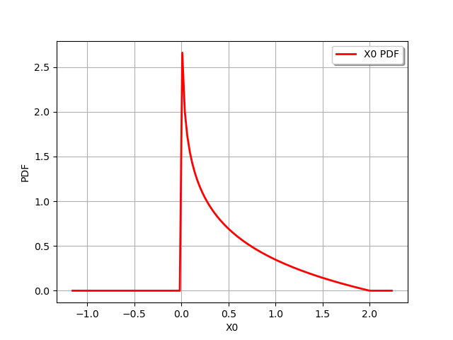
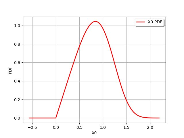
We might also compute the product of two (or more) distributions. For example :

distribution = distribution1 * distribution2
print(distribution)
graph = distribution.drawPDF()
view = viewer.View(graph)

Out:

ProductDistribution(Uniform(a = 0, b = 1) * Uniform(a = 0, b = 2))

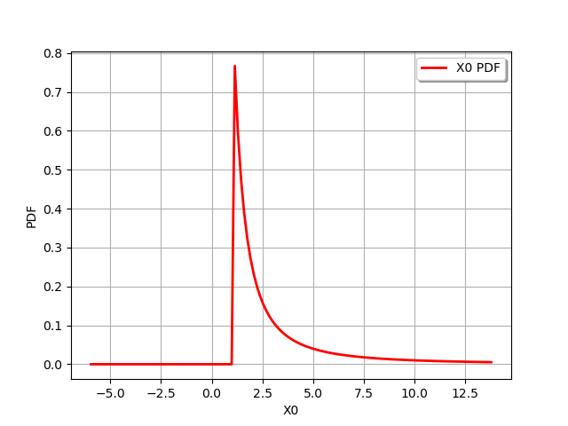
We could also inverse a distribution :

distribution = 1 / distribution1
print(distribution)
graph = distribution.drawPDF()
view = viewer.View(graph)

Out:

CompositeDistribution=f(Uniform(a = 0, b = 1)) with f=[x]->[1.0 / x]

Or compute a ratio distribution :

ratio = distribution2 / distribution1
print(ratio)
graph = ratio.drawPDF()
view = viewer.View(graph)

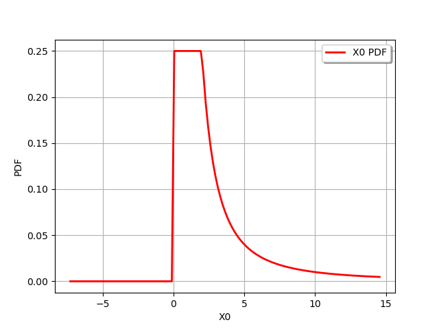
Out:

ProductDistribution(Uniform(a = 0, b = 2) * CompositeDistribution=f(Uniform(a = 0, b = 1)) with f=[x]->[1.0 / x])

Transformation using functions

The library provides methods to get the full distributions of f(x) where f can be equal to :

• sin,

• asin,

• cos,

• acos,

• tan,

• atan,

• sinh,

• asinh,

• cosh,

• acosh,

• tanh,

• atanh,

• sqr (for square),

• inverse,

• sqrt,

• exp,

• log/ln,

• abs,

• cbrt.

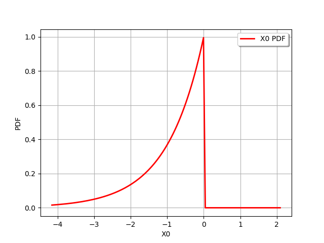
For example for the usual log transformation :

graph =distribution1.log().drawPDF()
view = viewer.View(graph)

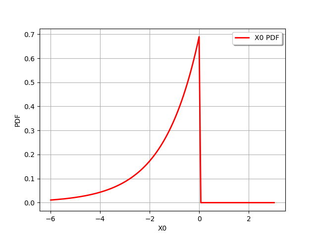
And for the log2 function :

f = ot.SymbolicFunction(['x'], ['log2(x)'])
f.setDescription(["X","ln(X)"])
graph = ot.CompositeDistribution(f, distribution1).drawPDF()
view = viewer.View(graph)

If one wants a specific method, user might rely on the CompositeDistribution class.

# Create a composite distribution
# -------------------------------
#
# In this paragraph we create a distribution defined as the push-forward distribution of a scalar distribution by a transformation.
#
# If we note :math:`\mathcal{L}_0` a scalar distribution, :math:`f: \mathbb{R} \rightarrow \mathbb{R}` a mapping, then it is possible to create the push-forward distribution :math:`\mathcal{L}` defined by
#
# .. math::
#    \mathcal{L} = f(\mathcal{L}_0)
#

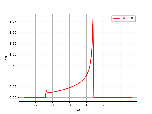
We create a 1D normal distribution :

antecedent = ot.Normal()

and a 1D transform :

f = ot.SymbolicFunction(['x'], ['sin(x)+cos(x)'])

We then create the composite distribution :

distribution = ot.CompositeDistribution(f, antecedent)
graph = distribution.drawPDF()
view = viewer.View(graph)

We can also build a distribution with the simplified construction :

distribution = antecedent.exp()
graph = distribution.drawPDF()
view = viewer.View(graph)

and by using chained operators :

distribution = antecedent.abs().sqrt()
graph = distribution.drawPDF()
view = viewer.View(graph)

Display all figures

plt.show()