Use the ANCOVA indices

In this example we are going to use the ANCOVA decomposition to estimate sensitivity indices from a model with correlated inputs.

ANCOVA allows to estimate the Sobol’ indices, and thanks to a functional decomposition of the model it allows to separate the part of variance explained by a variable itself from the part of variance explained by a correlation which is due to its correlation with the other input parameters.

In theory, ANCOVA indices range is ; the closer to 1 the index is, the greater the model response sensitivity to the variable is. These indices are a sum of a physical part and correlated part . The correlation has a weak influence on the contribution of , if is low and is close to . On the contrary, the correlation has a strong influence on the contribution of the input , if is high and is close to .

The ANCOVA indices evaluate the importance of one variable at a time ( indices stored, with the input dimension of the model). The uncorrelated parts of variance of the output due to each input and the effects of the correlation are represented by the indices resulting from the subtraction of these two previous lists.

To evaluate the indices, the library needs of a functional chaos result approximating the model response with uncorrelated inputs and a sample with correlated inputs used to compute the real values of the output.

from __future__ import print_function
import openturns as ot
import openturns.viewer as viewer
from matplotlib import pylab as plt
ot.Log.Show(ot.Log.NONE)

Create the model (x1,x2) –> (y) = (4.*x1+5.*x2)

model = ot.SymbolicFunction(['x1', 'x2'], ['4.*x1+5.*x2'])

Create the input independent joint distribution

distribution = ot.Normal(2)
distribution.setDescription(['X1', 'X2'])

Create the correlated input distribution

S = ot.CorrelationMatrix(2)
S[1, 0] = 0.3
R = ot.NormalCopula.GetCorrelationFromSpearmanCorrelation(S)
copula = ot.NormalCopula(R)
distribution_corr = ot.ComposedDistribution([ot.Normal()] * 2, copula)

ANCOVA needs a functional decomposition of the model

enumerateFunction = ot.LinearEnumerateFunction(2)
productBasis = ot.OrthogonalProductPolynomialFactory(
    [ot.HermiteFactory()]*2, enumerateFunction)
adaptiveStrategy = ot.FixedStrategy(
    productBasis, enumerateFunction.getStrataCumulatedCardinal(4))
samplingSize = 250
projectionStrategy = ot.LeastSquaresStrategy(
    ot.MonteCarloExperiment(samplingSize))
algo = ot.FunctionalChaosAlgorithm(
    model, distribution, adaptiveStrategy, projectionStrategy)
algo.run()
result = ot.FunctionalChaosResult(algo.getResult())

Create the input sample taking account the correlation

size = 2000
sample = distribution_corr.getSample(size)

Perform the decomposition

ancova = ot.ANCOVA(result, sample)
# Compute the ANCOVA indices (first order and uncorrelated indices are computed together)
indices = ancova.getIndices()
# Retrieve uncorrelated indices
uncorrelatedIndices = ancova.getUncorrelatedIndices()
# Retrieve correlated indices:
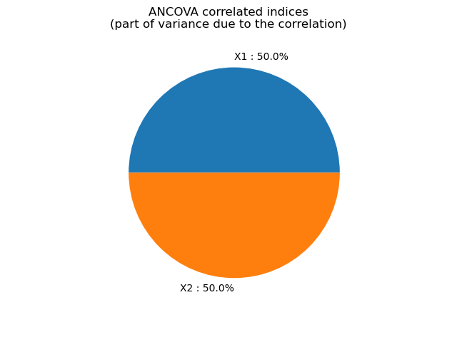
correlatedIndices = indices - uncorrelatedIndices

Print Sobol’ indices, the physical part, and the correlation part

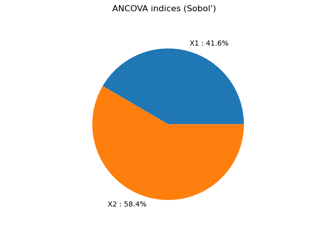
print("ANCOVA indices ", indices)
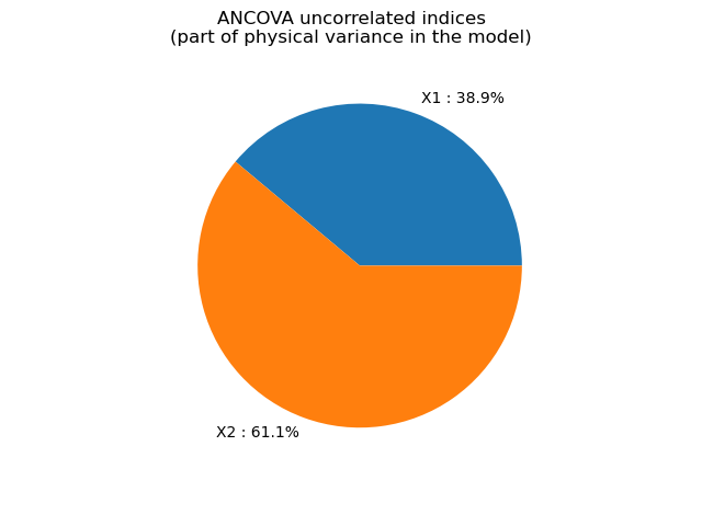
print("ANCOVA uncorrelated indices ", uncorrelatedIndices)
print("ANCOVA correlated indices ", correlatedIndices)

Out:

ANCOVA indices  [0.415841,0.584159]
ANCOVA uncorrelated indices  [0.295058,0.463375]
ANCOVA correlated indices  [0.120784,0.120784]

graph = ot.SobolIndicesAlgorithm.DrawImportanceFactors(
    indices, distribution.getDescription(), 'ANCOVA indices (Sobol\')')
view = viewer.View(graph)

graph = ot.SobolIndicesAlgorithm.DrawImportanceFactors(uncorrelatedIndices, distribution.getDescription(
), 'ANCOVA uncorrelated indices\n(part of physical variance in the model)')
view = viewer.View(graph)

graph = ot.SobolIndicesAlgorithm.DrawImportanceFactors(correlatedIndices, distribution.getDescription(
), 'ANCOVA correlated indices\n(part of variance due to the correlation)')
view = viewer.View(graph)
plt.show()