Calibration of the deflection of a tube

We calibrate the deflection of a tube as described here. More precisely, we calibrate the mechanical parameters of a model which computes the vertical deflection of a tube and two deflection angles. This example shows how to calibrate a computer code which has several outputs.

from openturns.usecases import deflection_tube
import openturns as ot
import openturns.viewer as viewer
from matplotlib import pylab as plt
ot.Log.Show(ot.Log.NONE)

Create a calibration problem

We load the model from the use case module :

dt = deflection_tube.DeflectionTube()

We create a sample out of our input distribution :

sampleSize = 100
inputSample = dt.inputDistribution.getSample(sampleSize)
inputSample[0:5]

	Force	Length	Location	External diameter	Internal diameter	Young Modulus
0	1.048972	1.5	1	0.8	0.1	201405.5
1	1.081729	1.5	1	0.8	0.1	198731.1
2	0.9955191	1.5	1	0.8	0.1	197684.8
3	1.026488	1.5	1	0.8	0.1	198344.6
4	0.9868583	1.5	1	0.8	0.1	197697.1

We take the image of our input sample by the model :

outputDeflection = dt.model(inputSample)
outputDeflection[0:5]

	Deflection	Left angle	Right angle
0	-7.197249e-06	-1.43945e-05	1.799312e-05
1	-7.521879e-06	-1.504376e-05	1.88047e-05
2	-6.959051e-06	-1.39181e-05	1.739763e-05
3	-7.151668e-06	-1.430334e-05	1.787917e-05
4	-6.898079e-06	-1.379616e-05	1.72452e-05

observationNoiseSigma = [0.1e-6, 0.05e-5, 0.05e-5]
observationNoiseCovariance = ot.CovarianceMatrix(3)
for i in range(3):
    observationNoiseCovariance[i, i] = observationNoiseSigma[i]**2

noiseSigma = ot.Normal([0., 0., 0.], observationNoiseCovariance)
sampleObservationNoise = noiseSigma.getSample(sampleSize)
observedOutput = outputDeflection + sampleObservationNoise
observedOutput[0:5]

	Deflection	Left angle	Right angle
0	-7.217769e-06	-1.512261e-05	1.82937e-05
1	-7.486931e-06	-1.500876e-05	1.885333e-05
2	-6.678776e-06	-1.283332e-05	1.780391e-05
3	-7.35846e-06	-1.402654e-05	1.791085e-05
4	-6.990384e-06	-1.370394e-05	1.742711e-05

observedInput = ot.Sample(sampleSize, 2)
observedInput[:, 0] = inputSample[:, 0]  # F
observedInput[:, 1] = inputSample[:, 5]  # E
observedInput.setDescription(["Force", "Young Modulus"])
observedInput[0:5]

	Force	Young Modulus
0	1.048972	201405.5
1	1.081729	198731.1
2	0.9955191	197684.8
3	1.026488	198344.6
4	0.9868583	197697.1

fullSample = ot.Sample(sampleSize, 5)
fullSample[:, 0:2] = observedInput
fullSample[:, 2:5] = observedOutput
fullSample.setDescription(
    ["Force", "Young", "Deflection", "Left Angle", "Right Angle"])
fullSample[0:5]

	Force	Young	Deflection	Left Angle	Right Angle
0	1.048972	201405.5	-7.217769e-06	-1.512261e-05	1.82937e-05
1	1.081729	198731.1	-7.486931e-06	-1.500876e-05	1.885333e-05
2	0.9955191	197684.8	-6.678776e-06	-1.283332e-05	1.780391e-05
3	1.026488	198344.6	-7.35846e-06	-1.402654e-05	1.791085e-05
4	0.9868583	197697.1	-6.990384e-06	-1.370394e-05	1.742711e-05

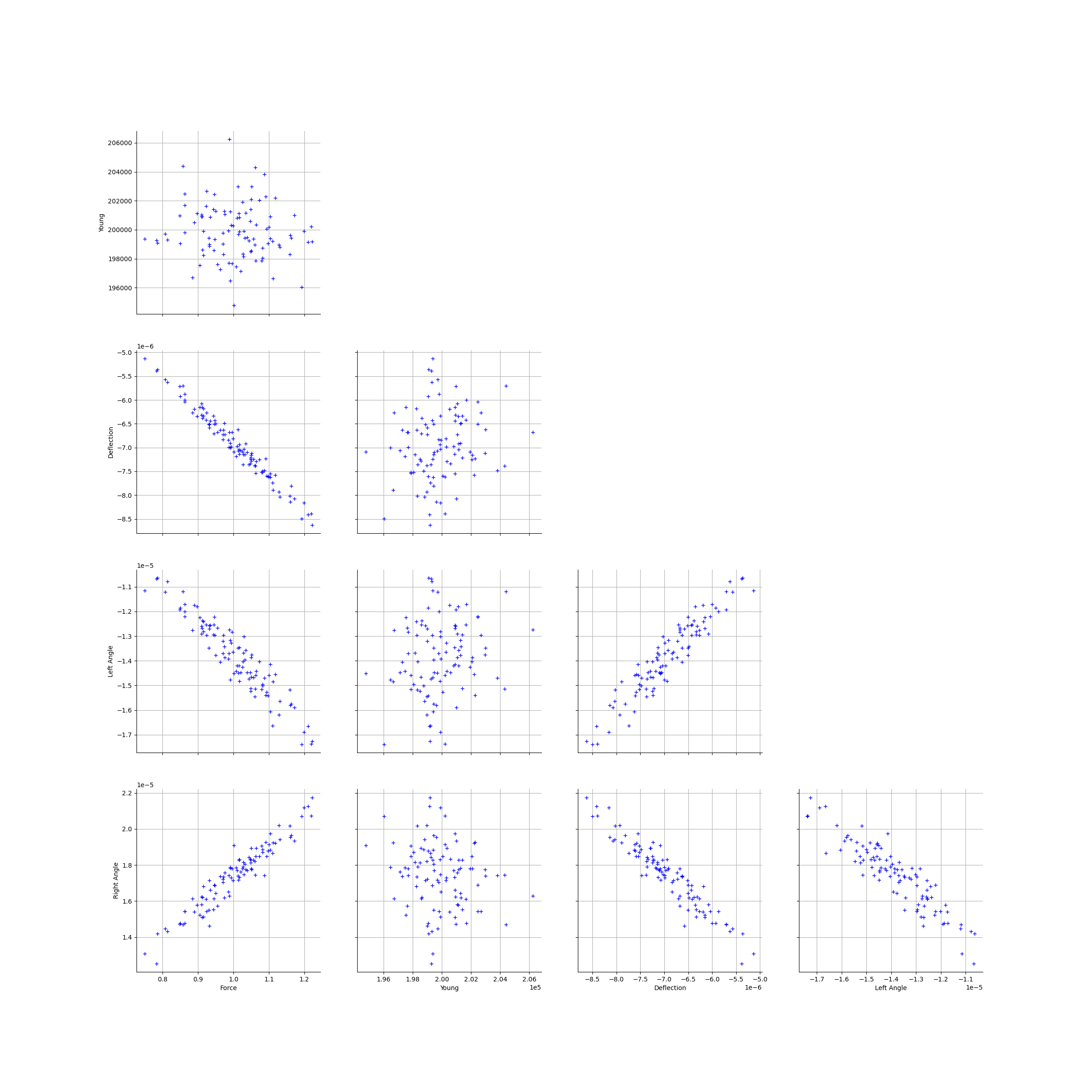
graph = ot.VisualTest.DrawPairs(fullSample)
view = viewer.View(graph)

Setting up the calibration

XL = 1.4  # Exact : 1.5
Xa = 1.2  # Exact : 1.0
XD = 0.7  # Exact : 0.8
Xd = 0.2  # Exact : 0.1
thetaPrior = [XL, Xa, XD, Xd]

sigmaXL = 0.1 * XL
sigmaXa = 0.1 * Xa
sigmaXD = 0.1 * XD
sigmaXd = 0.1 * Xd
parameterCovariance = ot.CovarianceMatrix(4)
parameterCovariance[0, 0] = sigmaXL**2
parameterCovariance[1, 1] = sigmaXa**2
parameterCovariance[2, 2] = sigmaXD**2
parameterCovariance[3, 3] = sigmaXd**2
parameterCovariance

[[ 0.0196 0 0 0 ]
[ 0 0.0144 0 0 ]
[ 0 0 0.0049 0 ]
[ 0 0 0 0.0004 ]]

calibratedIndices = [1, 2, 3, 4]
calibrationFunction = ot.ParametricFunction(
    dt.model, calibratedIndices, thetaPrior)

sigmaObservation = [0.2e-6, 0.03e-5, 0.03e-5]  # Exact : 0.1e-6

errorCovariance = ot.CovarianceMatrix(3)
errorCovariance[0, 0] = sigmaObservation[0]**2
errorCovariance[1, 1] = sigmaObservation[1]**2
errorCovariance[2, 2] = sigmaObservation[2]**2

calibrationFunction.setParameter(thetaPrior)
predictedOutput = calibrationFunction(observedInput)
predictedOutput[0:5]

	Deflection	Left angle	Right angle
0	-3.050547e-06	-1.016849e-05	1.65238e-05
1	-3.188141e-06	-1.062714e-05	1.72691e-05
2	-2.949587e-06	-9.831957e-06	1.597693e-05
3	-3.031228e-06	-1.010409e-05	1.641915e-05
4	-2.923744e-06	-9.745814e-06	1.583695e-05

Calibration with gaussian non linear least squares

algo = ot.GaussianNonLinearCalibration(
    calibrationFunction, observedInput, observedOutput, thetaPrior, parameterCovariance, errorCovariance)

algo.run()

calibrationResult = algo.getResult()

Analysis of the results

thetaMAP = calibrationResult.getParameterMAP()
thetaMAP

[1.50832,1.01261,0.801327,0.199875]

Compute a 95% confidence interval for each marginal.

thetaPosterior = calibrationResult.getParameterPosterior()
alpha = 0.95
dim = thetaPosterior.getDimension()
for i in range(dim):
    print(thetaPosterior.getMarginal(i).computeBilateralConfidenceInterval(alpha))

Out:

[1.48921, 1.52789]
[0.990035, 1.03407]
[0.797322, 0.80576]
[0.19985, 0.199926]

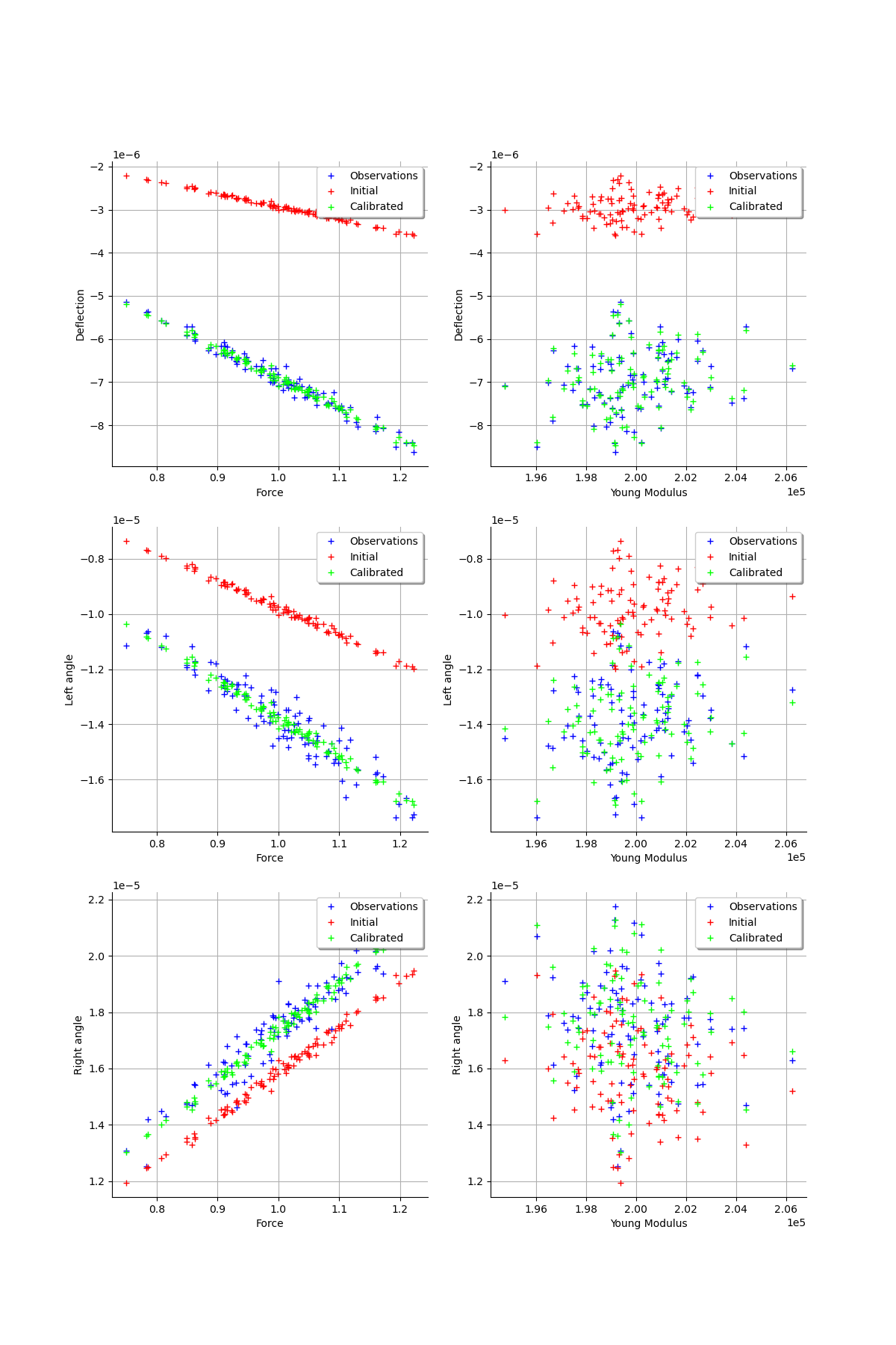
graph = calibrationResult.drawObservationsVsInputs()
view = viewer.View(graph)

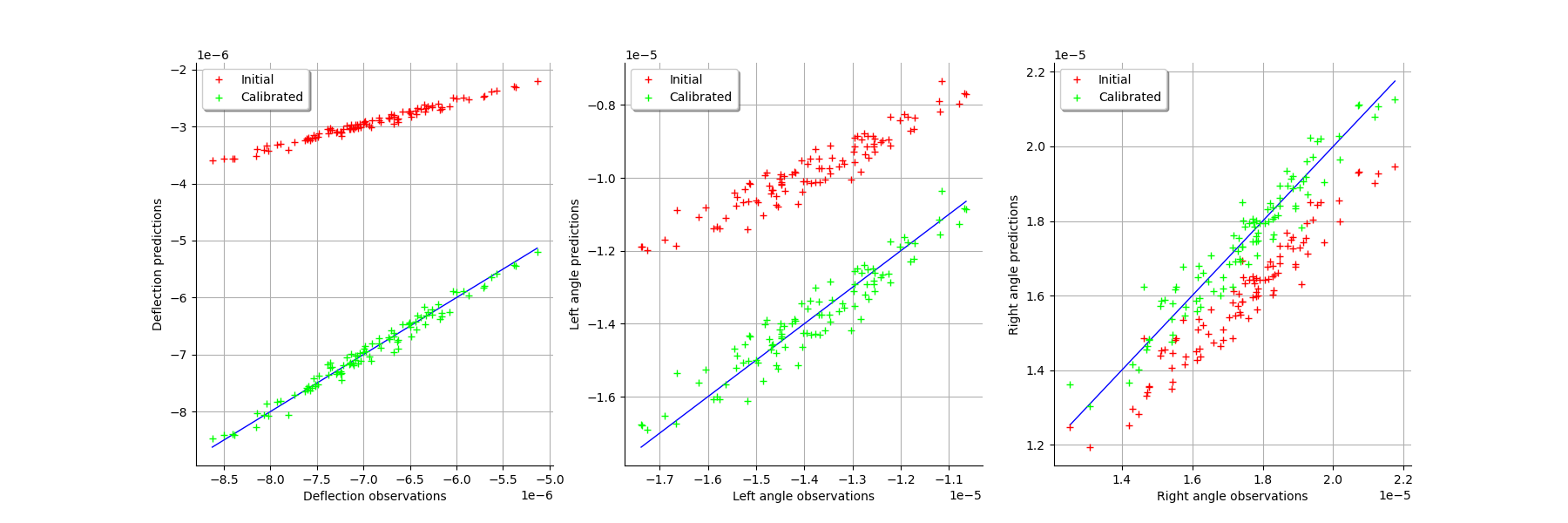
graph = calibrationResult.drawObservationsVsPredictions()
view = viewer.View(graph)

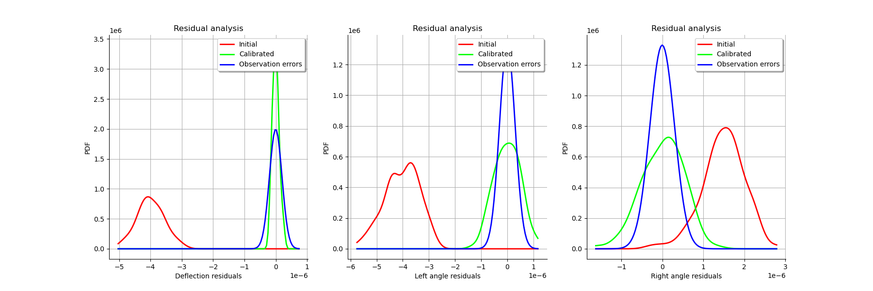
graph = calibrationResult.drawResiduals()
view = viewer.View(graph)

graph = calibrationResult.drawParameterDistributions()
view = viewer.View(graph)

plt.show()