Mixture of experts

In this example we are going to approximate a piece wise continuous function using an expert mixture of metamodels.

The metamodels will be represented by the family of :

where the N classes are defined by the classifier.

Using the supervised mode the classifier partitions the input and output space at once:

The classifier is MixtureClassifier based on a MixtureDistribution defined as:

The rule to assign a point to a class is defined as follows: is assigned to the class .

The grade of with respect to the class is .

import openturns as ot
from matplotlib import pyplot as plt
import openturns.viewer as viewer
from matplotlib import pylab as plt
from openturns.viewer import View
import numpy as np
ot.Log.Show(ot.Log.NONE)

dimension = 1

# Define the piecewise model we want to rebuild


def piecewise(X):
    # if x < 0.0:
    #     f = (x+0.75)**2-0.75**2
    # else:
    #     f = 2.0-x**2
    xarray = np.array(X, copy=False)
    return np.piecewise(xarray, [xarray < 0, xarray >= 0], [lambda x: x*(x+1.5), lambda x: 2.0 - x*x])


f = ot.PythonFunction(1, 1, func_sample=piecewise)

Build a metamodel over each segment

degree = 5
samplingSize = 100
enumerateFunction = ot.LinearEnumerateFunction(dimension)
productBasis = ot.OrthogonalProductPolynomialFactory(
    [ot.LegendreFactory()] * dimension, enumerateFunction)
adaptiveStrategy = ot.FixedStrategy(
    productBasis, enumerateFunction.getStrataCumulatedCardinal(degree))
projectionStrategy = ot.LeastSquaresStrategy(
    ot.MonteCarloExperiment(samplingSize))

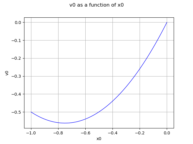
Segment 1: (-1.0; 0.0)

d1 = ot.Uniform(-1.0, 0.0)
fc1 = ot.FunctionalChaosAlgorithm(f, d1, adaptiveStrategy, projectionStrategy)
fc1.run()
mm1 = fc1.getResult().getMetaModel()
graph = mm1.draw(-1.0, -1e-6)
view = viewer.View(graph)

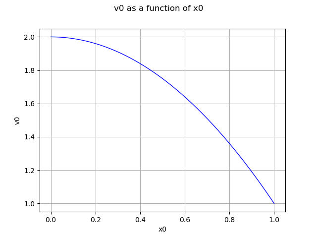
Segment 2: (0.0, 1.0)

d2 = ot.Uniform(0.0, 1.0)
fc2 = ot.FunctionalChaosAlgorithm(f, d2, adaptiveStrategy, projectionStrategy)
fc2.run()
mm2 = fc2.getResult().getMetaModel()
graph = mm2.draw(1e-6, 1.0)
view = viewer.View(graph)

Define the mixture

R = ot.CorrelationMatrix(2)
d1 = ot.Normal([-1.0, -1.0], [1.0]*2, R)  # segment 1
d2 = ot.Normal([1.0, 1.0], [1.0]*2, R)  # segment 2
weights = [1.0]*2
atoms = [d1, d2]
mixture = ot.Mixture(atoms, weights)

Create the classifier based on the mixture

classifier = ot.MixtureClassifier(mixture)

Create local experts using the metamodels

experts = ot.Basis([mm1, mm2])

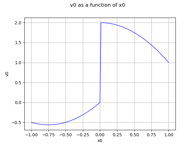
Create a mixture of experts

evaluation = ot.ExpertMixture(experts, classifier)
moe = ot.Function(evaluation)

Draw the mixture of experts

graph = moe.draw(-1.0, 1.0)
view = viewer.View(graph)
plt.show()