Kriging: metamodel of the Branin-Hoo function

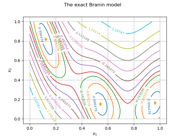
As a popular use case in optimization we briefly present the construction of a metamodel of the Branin (also referred to as Branin-Hoo) function.

from numpy import sqrt
import openturns as ot
import openturns.viewer as viewer
import openturns.viewer as otv
from openturns.usecases import branin_function
from matplotlib import pylab as plt

We load the Branin-Hoo model from the usecases module and use the model (stored in objectiveFunction)

bm = branin_function.BraninModel()
model = bm.objectiveFunction

We shall represent this 2D function with isolines. We set the number of isolines to a maximum of 10 thanks to the following ResourceMap key :

ot.ResourceMap.SetAsUnsignedInteger("Contour-DefaultLevelsNumber", 10)
graphBasic = model.draw([0.0, 0.0], [1.0, 1.0], [100]*2)

We get the values of all isolines :

drawables = graphBasic.getDrawables()
levels = []
for contours in drawables:
    levels.append(contours.getLevels()[0])

We now build fancy isolines :

# Take the first contour as the only one with multiple levels
contour = graphBasic.getDrawable(0)
# Build a range of colors
ot.ResourceMap.SetAsUnsignedInteger(
    'Drawable-DefaultPalettePhase', len(levels))
palette = ot.Drawable.BuildDefaultPalette(len(levels))
# Create the drawables list, appending each contour with its own color
drawables = list()
for i in range(len(levels)):
    contour.setLevels([levels[i]])
    # Inline the level values
    contour.setDrawLabels(True)
    # We have to copy the drawable because a Python list stores only pointers
    drawables.append(ot.Drawable(contour))

graphFineTune = ot.Graph("The exact Branin model",
                         r"$x_1$", r"$x_2$", True, '')
graphFineTune.setDrawables(drawables)  # Replace the drawables
graphFineTune.setLegendPosition("")  # Remove the legend
graphFineTune.setColors(palette)  # Add colors

We also represent the three minima of the Branin function with orange diamonds :

sample1 = ot.Sample([bm.xexact1, bm.xexact2, bm.xexact3])
cloud1 = ot.Cloud(sample1, 'orange', 'diamond', 'First Cloud')
graphFineTune.add(cloud1)
view = otv.View(graphFineTune)

#
# The values of the exact model at these points are :
print(bm.objectiveFunction(sample1))

Out:

    [ y0       ]
0 : [ -1.04741 ]
1 : [ -1.04741 ]
2 : [ -1.04741 ]

The Branin function has a global minimum attained at three different points. We shall build a metamodel of this function that presents the same behaviour.

Definition of the Kriging metamodel

We use the KrigingAlgorithm class to perform the kriging analysis. We first generate a design of experiments with LHS and store the input trainig points in xdata

experiment = ot.LHSExperiment(ot.ComposedDistribution(
    [ot.Uniform(0.0, 1.0), ot.Uniform(0.0, 1.0)]), 28, False, True)
xdata = experiment.generate()

We also get the output training values :

ydata = bm.objectiveFunction(xdata)

This use case is defined in dimension 2 and we use a constant basis for the trend estimation :

dimension = bm.dim
basis = ot.ConstantBasisFactory(dimension).build()

We choose a squared exponential covariance model in dimension 2 :

covarianceModel = ot.SquaredExponential([0.1]*dimension, [1.0])

We have all the components to build a kriging algorithm and run it :

algo = ot.KrigingAlgorithm(xdata, ydata, covarianceModel, basis)
algo.run()

We get the result of the kriging analysis with :

result = algo.getResult()

Metamodel visualization

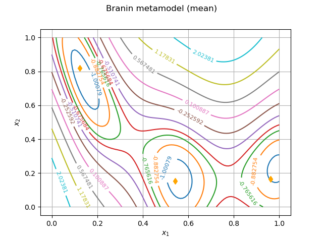
We draw the kriging metamodel of the Branin function. It is the mean of the random process.

metamodel = result.getMetaModel()


graphBasic = metamodel.draw([0.0, 0.0], [1.0, 1.0], [100]*2)
drawables = graphBasic.getDrawables()
levels = []
for i in range(len(drawables)):
    contours = drawables[i]
    levels.append(contours.getLevels()[0])

# Take the first contour as the only one with multiple levels
contour = graphBasic.getDrawable(0)
# Build a range of colors
ot.ResourceMap.SetAsUnsignedInteger(
    'Drawable-DefaultPalettePhase', len(levels))
palette = ot.Drawable.BuildDefaultPalette(len(levels))
# Create the drawables list, appending each contour with its own color
drawables = list()
for i in range(len(levels)):
    contour.setLevels([levels[i]])
    # Inline the level values
    contour.setDrawLabels(True)
    # We have to copy the drawable because a Python list stores only pointers
    drawables.append(ot.Drawable(contour))

graphFineTune = ot.Graph("Branin metamodel (mean)",
                         r"$x_1$", r"$x_2$", True, '')
graphFineTune.setDrawables(drawables)
graphFineTune.setLegendPosition("")
graphFineTune.setColors(palette)

We also represent the location of the minima of the Branin function :

sample1 = ot.Sample([bm.xexact1, bm.xexact2, bm.xexact3])
cloud1 = ot.Cloud(sample1, 'orange', 'diamond', 'First Cloud')
graphFineTune.add(cloud1)
view = otv.View(graphFineTune)

We evaluate the metamodel at the minima locations :

print(metamodel(sample1))

Out:

0 : [ -1.06289 ]
1 : [ -1.0503  ]
2 : [ -1.0058  ]

Graphically, both the metamodel and the exact function look the same. The metamodel also has three basins around the minima and the value of the metamodel at each minimum location is comparable to the exact value of -0.979476. We have roughly two correct digits for each isoline.

Standard deviation

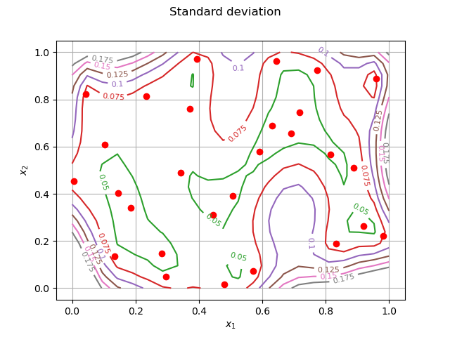
We finally take a look at the standard deviation in the domain. It may be seen as a measure of the error of the metamodel.

We discretize the domain with 22 points (N inside points and 2 endpoints) :

N = 20
inputData = ot.Box([N, N]).generate()

We compute the conditional variance of the model and take the square root to get the deviation :

condCov = result.getConditionalMarginalVariance(inputData, 0)
condCovSd = sqrt(condCov)

As we have previously done we build contours with the following levels ans labels :

levels = [0.01, 0.025, 0.050, 0.075, 0.1, 0.125, 0.150, 0.175]
labels = ['0.01', '0.025', '0.050', '0.075', '0.1', '0.125', '0.150', '0.175']
contour = ot.Contour(N+2, N+2, condCovSd)
graph = ot.Graph('', 'x', 'y', True, '')
graph.add(contour)

We use fancy colored isolines for the contour plot :

contour = graph.getDrawable(0)
ot.ResourceMap.SetAsUnsignedInteger(
    'Drawable-DefaultPalettePhase', len(levels))
palette = ot.Drawable.BuildDefaultPalette(len(levels))
drawables = list()
for i in range(len(levels)):
    contour.setLevels([levels[i]])
    contour.setDrawLabels(True)
    drawables.append(ot.Drawable(contour))

graphFineTune = ot.Graph("Standard deviation", r"$x_1$", r"$x_2$", True, '')
graphFineTune.setDrawables(drawables)
graphFineTune.setLegendPosition("")
graphFineTune.setColors(palette)

We superimpose the training sample :

cloud = ot.Cloud(xdata)
cloud.setPointStyle("fcircle")
cloud.setColor("red")
graphFineTune.add(cloud)
view = otv.View(graphFineTune)

We observe that the standard deviation is small in the center of the domain where we have enough data to learn the model. We can print the value of the variance at the first 5 training points (they all behave similarly) :

print(result.getConditionalMarginalVariance(xdata, 0)[0:5])

Out:

    [ v0         ]
0 : [ 0.00346411 ]
1 : [ 0.00361334 ]
2 : [ 0.003614   ]
3 : [ 0.00176519 ]
4 : [ 0.00287703 ]

These values are nearly zero which is expected as the kriging interpolates data. The value being known it is not random anymore and the variance ought to be zero.

Display all figures

plt.show()