Note
Click here to download the full example code
Create a functional basis process
The objective of this example is to define
a multivariate stochastic
process of dimension
where
, as a linear
combination of
deterministic functions
:
where is a random vector of dimension
.
We suppose that is discretized on the mesh
which has
vertices.
A realization of on
consists in generating a realization
of the random vector
and in evaluating the
functions
on the mesh
.
If we note
the realization of
, where
, we have:
import openturns as ot
import openturns.viewer as viewer
from matplotlib import pylab as plt
import math as m
ot.Log.Show(ot.Log.NONE)
Define the coefficients distribution
mu = [2.0]*2
sigma = [5.0]*2
R = ot.CorrelationMatrix(2)
coefDist = ot.Normal(mu, sigma, R)
Create a basis of functions
phi_1 = ot.SymbolicFunction(['t'], ['sin(t)'])
phi_2 = ot.SymbolicFunction(['t'], ['cos(t)^2'])
myBasis = ot.Basis([phi_1, phi_2])
Create the mesh
myMesh = ot.RegularGrid(0.0, 0.1, 100)
Create the process
process = ot.FunctionalBasisProcess(coefDist, myBasis, myMesh)
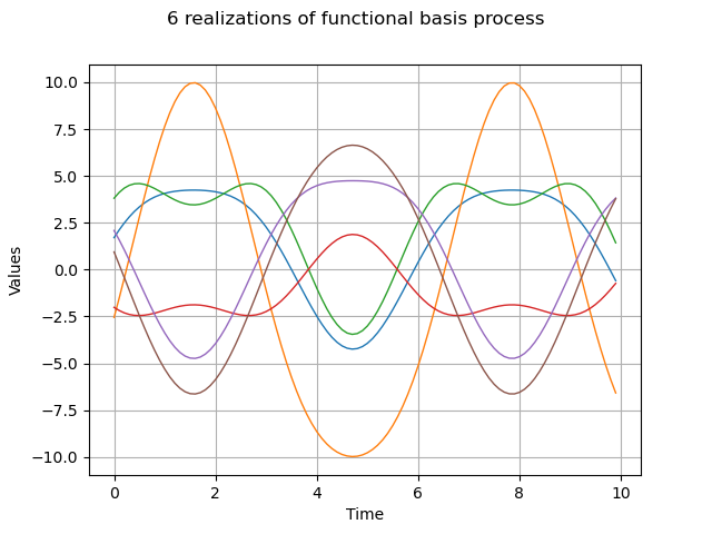
Draw a sample
N = 6
sample = process.getSample(N)
graph = sample.drawMarginal(0)
graph.setTitle(str(N)+' realizations of functional basis process')
view = viewer.View(graph)

Total running time of the script: ( 0 minutes 0.074 seconds)
 OpenTURNS