Note
Click here to download the full example code
Time variant system reliability problem
The objective is to evaluate the outcrossing rate from a safe to a failure domain in a time variant reliability problem.
We consider the following limit state function, defined as the difference between a degrading resistance and a time-varying load
:
- ..math:
begin{align*} g(t)= r(t) - S(t) = R - bt - S(t) quad forall t in [0,T] end{align*}
The failure domaine is defined by:
which means that the resistance at is less thant the stress at
.
We propose the following probabilistic model:
is the initial resistance, and
;
is the deterioration rate of the resistance; it is deterministic;
is the time-varying stress, which is modeled by a stationary Gaussian process of mean value
, standard deviation
and a squared exponential covariance model
.
The outcrossing rate from the safe to the failure domain at instant is defined by:
For each , we note the random variable
where
.
To evaluate , we need to consider the bivariate random vector
.
The event writes as the intersection of both events :
and
.
The objective is to evaluate:
1. Define some useful functions
We define the bivariate random vector .
Here,
is a bivariate Normal random vector:
whith mean
and
whith covariance matrix
defined by:
- ..math::
begin{align*} Sigma = left( begin{array}{cc} C(t, t) & C(t, t+Delta t) \ C(t, t+Delta t) & C(t+Delta t, t+Delta t) end{array} right) end{align*}
This function buils .
from math import sqrt
from openturns.viewer import View
from openturns import *


def buildNormal(b, t, mu_S, covariance, delta_t=1e-5):
    sigma = CovarianceMatrix(2)
    sigma[0, 0] = covariance(t, t)[0, 0]
    sigma[0, 1] = covariance(t, t+delta_t)[0, 0]
    sigma[1, 1] = covariance(t+delta_t, t+delta_t)[0, 0]
    return Normal([b*t + mu_S, b*(t+delta_t) + mu_S], sigma)
This function creates the trivariate random vector where
is independent from
. We need to create this random vector because both events
and
must be defined from the same random vector!
def buildCrossing(b, t, mu_S, covariance, R, delta_t=1e-5):
    normal = buildNormal(b, t, mu_S, covariance, delta_t)
    # return BlockIndependentDistribution([R, normal]): only from the 1.16 version!
    marg = [R, normal.getMarginal(0), normal.getMarginal(1)]
    cop = ComposedCopula([IndependentCopula(1), normal.getCopula()])
    return ComposedDistribution(marg, cop)
This function evaluates the probability using the Monte Carlo sampling. It defines the intersection event .
def computeCrossingProbability_MonteCarlo(b, t, mu_S, covariance, R, delta_t, n_block, n_iter, CoV):
    full = buildCrossing(b, t, mu_S, covariance, R, delta_t)
    X = RandomVector(full)
    f1 = SymbolicFunction(["R", "X1", "X2"], ["X1 - R"])
    e1 = ThresholdEvent(CompositeRandomVector(f1, X), Less(), 0.0)
    f2 = SymbolicFunction(["R", "X1", "X2"], ["X2 - R"])
    e2 = ThresholdEvent(CompositeRandomVector(f2, X), GreaterOrEqual(), 0.0)
    event = IntersectionEvent([e1, e2])
    algo = ProbabilitySimulationAlgorithm(event, MonteCarloExperiment())
    algo.setBlockSize(n_block)
    algo.setMaximumOuterSampling(n_iter)
    algo.setMaximumCoefficientOfVariation(CoV)
    algo.run()
    return algo.getResult().getProbabilityEstimate() / delta_t
This function evaluates the probability using the Low Discrepancy sampling.
def computeCrossingProbability_QMC(b, t, mu_S, covariance, R, delta_t, n_block, n_iter, CoV):
    full = buildCrossing(b, t, mu_S, covariance, R, delta_t)
    X = RandomVector(full)
    f1 = SymbolicFunction(["R", "X1", "X2"], ["X1 - R"])
    e1 = ThresholdEvent(CompositeRandomVector(f1, X), Less(), 0.0)
    f2 = SymbolicFunction(["R", "X1", "X2"], ["X2 - R"])
    e2 = ThresholdEvent(CompositeRandomVector(f2, X), GreaterOrEqual(), 0.0)
    event = IntersectionEvent([e1, e2])
    algo = ProbabilitySimulationAlgorithm(event, LowDiscrepancyExperiment(
        SobolSequence(X.getDimension()), n_block, False))
    algo.setBlockSize(n_block)
    algo.setMaximumOuterSampling(n_iter)
    algo.setMaximumCoefficientOfVariation(CoV)
    algo.run()
    return algo.getResult().getProbabilityEstimate() / delta_t
This function evaluates the probability using the FORM algorithm for event systems..
def computeCrossingProbability_FORM(b, t, mu_S, covariance, R, delta_t):
    full = buildCrossing(b, t, mu_S, covariance, R, delta_t)
    X = RandomVector(full)
    f1 = SymbolicFunction(["R", "X1", "X2"], ["X1 - R"])
    e1 = ThresholdEvent(CompositeRandomVector(f1, X), Less(), 0.0)
    f2 = SymbolicFunction(["R", "X1", "X2"], ["X2 - R"])
    e2 = ThresholdEvent(CompositeRandomVector(f2, X), GreaterOrEqual(), 0.0)
    event = IntersectionEvent([e1, e2])
    algo = SystemFORM(SQP(), event, X.getMean())
    algo.run()
    return algo.getResult().getEventProbability() / delta_t
2. Evaluate the probability
First, fix some parameters: and the covariance model which is the Squared Exponential model.
Be careful to the parameter
which is of great importance: if it is too small, the simulation methods have problems to converge because the correlation rate is too high between the instants
and
.
We advice to take
.
mu_S = 3.0
sigma_S = 0.5
l = 10

b = 0.01

mu_R = 5.0
sigma_R = 0.3
R = Normal(mu_R, sigma_R)

covariance = SquaredExponential([l/sqrt(2)], [sigma_S])

t0 = 0.0
t1 = 50.0
N = 26

# Get all the time steps t
times = RegularGrid(t0, (t1 - t0) / (N - 1.0), N).getVertices()

delta_t = 1e-1
Use all the methods previously described:
Monte Carlo: values in values_MC
Low discrepancy suites: values in values_QMC
FORM: values in values_FORM
values_MC = list()
values_QMC = list()
values_FORM = list()

for tick in times:
    values_MC.append(computeCrossingProbability_MonteCarlo(
        b, tick[0], mu_S, covariance, R, delta_t, 2**12, 2**3, 1e-2))
    values_QMC.append(computeCrossingProbability_QMC(
        b, tick[0], mu_S, covariance, R, delta_t, 2**12, 2**3, 1e-2))
    values_FORM.append(computeCrossingProbability_FORM(
        b, tick[0], mu_S, covariance, R, delta_t))
print('Values MC = ', values_MC)
print('Values QMC = ', values_QMC)
print('Values FORM = ', values_FORM)
Out:
Values MC =  [0.0, 0.00030517578125, 0.0, 0.0, 0.00030517578125, 0.00030517578125, 0.00030517578125, 0.0, 0.00030517578125, 0.0, 0.0, 0.0, 0.0, 0.0, 0.0, 0.00030517578125, 0.00030517578125, 0.00030517578125, 0.00091552734375, 0.00030517578125, 0.0, 0.00030517578125, 0.0006103515625, 0.0006103515625, 0.00091552734375, 0.00091552734375]
Values QMC =  [0.0, 0.0, 0.0, 0.0, 0.0, 0.0, 0.0006103515625, 0.0, 0.0006103515625, 0.0, 0.0, 0.0, 0.00030517578125, 0.00030517578125, 0.0, 0.00030517578125, 0.0, 0.00091552734375, 0.0006103515625, 0.0, 0.00030517578125, 0.0, 0.0006103515625, 0.001220703125, 0.00091552734375, 0.0006103515625]
Values FORM =  [6.407247221452685e-05, 7.202731340860951e-05, 8.087457491593016e-05, 9.070179169300293e-05, 0.0001016035263802752, 0.00011368175169084065, 0.00012704623305305574, 0.00014181490835112135, 0.00015811426182631293, 0.00017607968850372457, 0.00019585584543730799, 0.00021759698560570485, 0.0002414672698574692, 0.00026764105252706364, 0.0002963031350828803, 0.0003276489830651007, 0.00036188490016252284, 0.00039922815388919713, 0.00043990704675780126, 0.00048416092659680056, 0.0005322401297909951, 0.0005844058510196042, 0.0006409299329991489, 0.0007020945699336272, 0.0007681919182910387, 0.0008395236089949951]
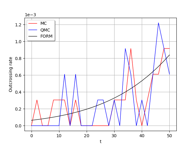
Draw the graphs!
g = Graph()
g.setAxes(True)
g.setGrid(True)
c = Curve(times, [[p] for p in values_MC])
g.add(c)
c = Curve(times, [[p] for p in values_QMC])
g.add(c)
c = Curve(times, [[p] for p in values_FORM])
g.add(c)
g.setLegends(["MC", "QMC", "FORM"])
g.setColors(["red", "blue", 'black'])
g.setLegendPosition("topleft")
g.setXTitle("t")
g.setYTitle("Outcrossing rate")
view = View(g)
view.ShowAll()

Total running time of the script: ( 0 minutes 5.444 seconds)
 OpenTURNS