Uncertainty ranking: Pearson’s correlation
This method deals with analyzing the influence the random vector
has on a random
variable
which is being studied for uncertainty. Here we
attempt to measure linear relationships that exist between
and the different components
.
Pearson’s correlation coefficient , defined in ,
measures the strength of a linear relation between two random variables
and
. If we have a sample made up of
pairs
,
, …,
, we can obtain
an
estimation of Pearson’s coefficient. The hierarchical ordering of
Pearson’s coefficients is of interest in the case where the relationship
between
and
variables
is close to being a linear
relation:
To obtain an indication of the role played by each in the
dispersion of
, the idea is to estimate Pearson’s correlation
coefficient
for each
. One can
then order the
variables
taking
absolute values of the correlation coefficients: the higher the value of
the greater the impact
the variable
has on the dispersion of
.
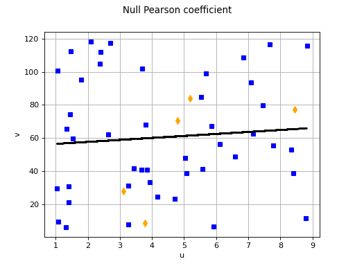
(Source code, png, hires.png, pdf)

API:
See
HypothesisTest_Pearson()
Examples:
References:
Saltelli, A., Chan, K., Scott, M. (2000). “Sensitivity Analysis”, John Wiley & Sons publishers, Probability and Statistics series
J.C. Helton, F.J. Davis (2003). “Latin Hypercube sampling and the propagation of uncertainty analyses of complex systems”. Reliability Engineering and System Safety 81, p.23-69
J.P.C. Kleijnen, J.C. Helton (1999). “Statistical analyses of scatterplots to identify factors in large-scale simulations, part 1 : review and comparison of techniques”. Reliability Engineering and System Safety 65, p.147-185
 OpenTURNS