Example of multi output Kriging on the fire satellite model

This example aims to illustrate Kriging metamodel with several outputs on the fire satellite model.

Loading of the model

This model involves 9 input variables and 3 output variables. We load the Fire satellite use case.

import openturns as ot
from openturns.usecases.fireSatellite_function import FireSatelliteModel
from openturns.viewer import View

ot.Log.Show(ot.Log.NONE)

m = FireSatelliteModel()

We define the function that evaluates the outputs depending on the inputs.

model = m.model

We also define the distribution of input variables to build the training and test sets.

inputDistribution = m.distributionX

Generation of data

We now generate the input and output training sets as 10 times the dimension of the input vector.

experiment = ot.LHSExperiment(inputDistribution, 10 * m.dim)
inputTrainingSet = experiment.generate()
outputTrainingSet = model(inputTrainingSet)

print("Lower and upper bounds of inputTrainingSet:")
print(inputTrainingSet.getMin(), inputTrainingSet.getMax())

Lower and upper bounds of inputTrainingSet:
[1.55043e+07,858.384,1348.18,12.1472,0.941856,-2.36658,2.56668,1.00003,0.13223] [2.03652e+07,1124.9,1450.72,18.4199,3.23979,2.93037,7.7944,2.93353,1.98141]

Creation of metamodel

We choose to use a constant trend.

basis = ot.ConstantBasisFactory(m.dim).build()

We would like to have separate covariance models for the three outputs. To do so, we use the TensorizedCovarianceModel. For the purpose of illustration, we consider MaternModel for the first and third outputs, and SquaredExponential for the second output.

myCov1 = ot.MaternModel([1.0] * m.dim, 2.5)
myCov2 = ot.SquaredExponential([1.0] * m.dim)
myCov3 = ot.MaternModel([1.0] * m.dim, 2.5)

covarianceModel = ot.TensorizedCovarianceModel([myCov1, myCov2, myCov3])

The scaling of the data is really important when dealing with Kriging, especially considering the domain definition of the input variables (the altitude varies in order of 1e7 whereas the drag coefficient is around 1). We thus define appropriate bounds for the training algorithm based on the domain definition of each variable.

scaleOptimizationBounds = ot.Interval(
    [1.0, 1.0, 0.1, 0.01, 0.1, 0.1, 0.01, 0.01, 0.001, 0.01, 0.01, 0.01],
    [1.0e7, 2.0e3, 2.0e3, 1e2, 10.0, 10.0, 10.0, 10.0, 10.0, 1e8, 1e4, 1e3],
)

We can now define the scaled version of Kriging model.

covarianceModel.setScale(inputTrainingSet.getMax())
algo = ot.KrigingAlgorithm(inputTrainingSet, outputTrainingSet, covarianceModel, basis)
algo.setOptimizationBounds(scaleOptimizationBounds)

We run the algorithm and get the metamodel.

algo.run()
result = algo.getResult()
krigingMetamodel = result.getMetaModel()

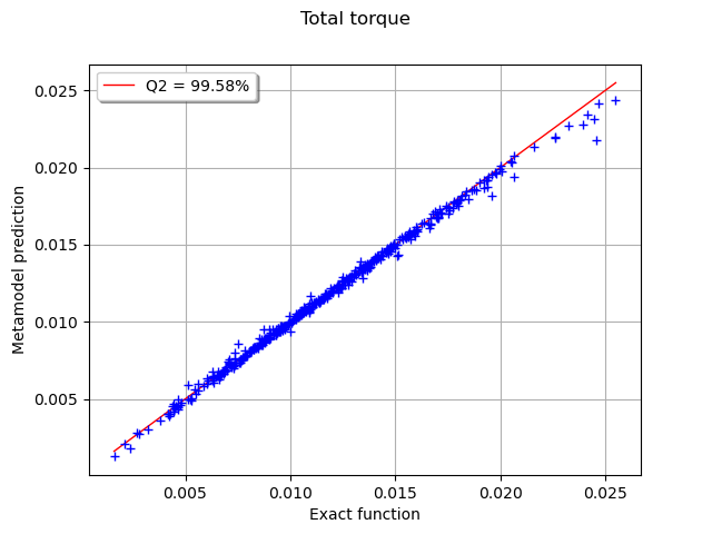
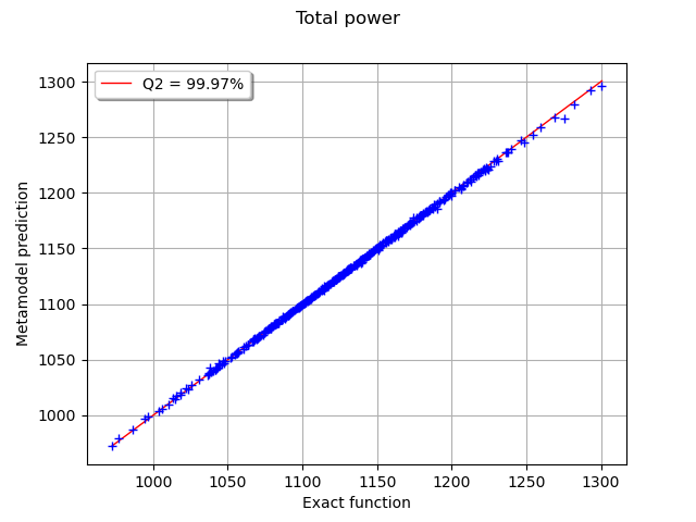
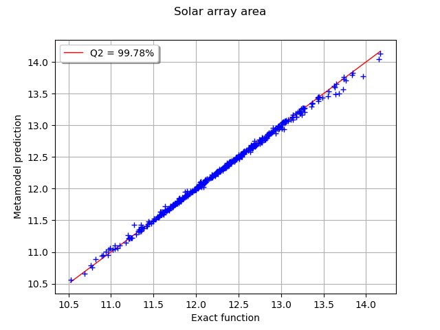
Validation of metamodel

To validate the metamodel, we create a validation set of size equal to 50 times the input vector dimension to evaluate the functions.

experimentTest = ot.LHSExperiment(inputDistribution, 50 * m.dim)
inputTestSet = experimentTest.generate()
outputTestSet = model(inputTestSet)
outputKriging = krigingMetamodel(inputTestSet)

Then, we use the MetaModelValidation class to validate the metamodel.

val = ot.MetaModelValidation(inputTestSet, outputTestSet, krigingMetamodel)

Q2 = val.computePredictivityFactor()

label = ["Total torque", "Total power", "Solar array area"]

for i in range(3):
    graph = val.drawValidation().getGraph(0, i)
    graph.setLegends([""])
    graph.setLegends(["Q2 = %.2f%%" % (100 * Q2[i]), ""])
    graph.setLegendPosition("topleft")
    graph.setXTitle("Exact function")
    graph.setYTitle("Metamodel prediction")
    graph.setTitle(label[i])
    View(graph)

• 
• 
•