Chaos cross-validation¶

In this example, we show how to perform the cross-validation of the Ishigami model using polynomial chaos expansion. More precisely, we use the methods suggested in [muller2016], chapter 5, page 257. We make the assumption that a dataset is given and we create a metamodel using this data. Once done, we want to assess the quality of the metamodel using the data we have.

We compare several methods:

split the data into two subsets, one for training and one for testing,
use k-fold validation.

The split of the data is performed by the compute_Q2_score_by_splitting function below. It uses 75% of the data to estimate the coefficients of the metamodel (this is the training step) and use 25% of the data to estimate the $Q^2$ score (this is the validation step). To do this, we use the split method of the Sample.

The K-Fold validation is performed by the compute_Q2_score_by_kfold function below. It uses the K-Fold method with $k = 5$ . The code uses the KFoldSplitter class, which computes the appropriate indices. Similar results can be obtained with LeaveOneOutSplitter at a higher cost.

This cross-validation method is used here to see which polynomial degree leads to an accurate metamodel of the Ishigami test function.

import openturns as ot
import openturns.viewer as otv
from openturns.usecases import ishigami_function

def compute_sparse_least_squares_chaos(
    inputTrain, outputTrain, basis, totalDegree, distribution
):
    """
    Create a sparse polynomial chaos based on least squares.

    * Uses the enumerate rule in basis.
    * Uses the LeastSquaresStrategy to compute the coefficients based on
      least squares.
    * Uses LeastSquaresMetaModelSelectionFactory to use the LARS selection method.
    * Uses FixedStrategy in order to keep all the coefficients that the
      LARS method selected.

    Parameters
    ----------
    inputTrain : Sample
        The input design of experiments.
    outputTrain : Sample
        The output design of experiments.
    basis : Basis
        The multivariate chaos basis.
    totalDegree : int
        The total degree of the chaos polynomial.
    distribution : Distribution.
        The distribution of the input variable.

    Returns
    -------
    result : PolynomialChaosResult
        The estimated polynomial chaos.
    """
    selectionAlgorithm = ot.LeastSquaresMetaModelSelectionFactory()
    projectionStrategy = ot.LeastSquaresStrategy(
        inputTrain, outputTrain, selectionAlgorithm
    )
    enumfunc = basis.getEnumerateFunction()
    P = enumfunc.getStrataCumulatedCardinal(totalDegree)
    adaptiveStrategy = ot.FixedStrategy(basis, P)
    chaosalgo = ot.FunctionalChaosAlgorithm(
        inputTrain, outputTrain, distribution, adaptiveStrategy, projectionStrategy
    )
    chaosalgo.run()
    result = chaosalgo.getResult()
    return result

def compute_Q2_score_by_splitting(
    X, Y, basis, totalDegree, distribution, split_fraction=0.75
):
    """
    Compute Q2 score by splitting into train/test sets.

    Parameters
    ----------
    X : Sample(size, input_dimension)
        The X dataset.
    Y : Sample(size, output_dimension)
        The Y dataset.

    Returns
    -------
    Q2_score : float
        The Q2 score.
    """

    training_sample_size = X.getSize()
    X_train = ot.Sample(X)
    Y_train = ot.Sample(Y)
    split_index = int(split_fraction * training_sample_size)
    X_test = X_train.split(split_index)
    Y_test = Y_train.split(split_index)
    result = compute_sparse_least_squares_chaos(
        X_train, Y_train, basis, totalDegree, distribution
    )
    metamodel = result.getMetaModel()
    val = ot.MetaModelValidation(X_test, Y_test, metamodel)
    Q2_score = val.computePredictivityFactor()[0]
    return Q2_score

def compute_Q2_score_by_kfold(X, Y, basis, totalDegree, distribution, n_folds=5):
    """
    Compute score by KFold.

    Parameters
    ----------
    X : Sample(size, input_dimension)
        The X dataset.
    Y : Sample(size, output_dimension)
        The Y dataset.

    Returns
    -------
    Q2_score : float
        The Q2 score.
    """
    #
    training_sample_size = X.getSize()
    splitter = ot.KFoldSplitter(training_sample_size, n_folds)
    Q2_score_list = ot.Sample(0, 1)
    for indices1, indices2 in splitter:
        X_train, X_test = X[indices1], X[indices2]
        Y_train, Y_test = Y[indices1], Y[indices2]
        result = compute_sparse_least_squares_chaos(
            X_train, Y_train, basis, totalDegree, distribution
        )
        metamodel = result.getMetaModel()
        val = ot.MetaModelValidation(X_test, Y_test, metamodel)
        Q2_local = val.computePredictivityFactor()[0]
        Q2_score_list.add([Q2_local])
    Q2_score = Q2_score_list.computeMean()[0]
    return Q2_score

We start by generating the input and output sample. We use a sample size equal to 1000.

im = ishigami_function.IshigamiModel()
im.distributionX.setDescription(["$X_0$", "$X_1$", "$X_2$"])
im.model.setOutputDescription(["$Y$"])
ot.RandomGenerator.SetSeed(0)
sample_size = 1000
X = im.distributionX.getSample(sample_size)
print("Input sample:")
print(X[:5])
Y = im.model(X)
Y.setDescription(["$Y$"])
print("Output sample:")
print(Y[:5])

Input sample:
    [ $X_0$     $X_1$     $X_2$     ]
: [  0.816038  2.67553   0.501506 ]
: [  2.40524  -2.19212  -0.705186 ]
: [ -2.29163   1.30032  -1.41281  ]
: [ -2.93737  -0.733649  2.30831  ]
: [ -0.960969 -0.43361  -2.39129  ]
Output sample:
    [ $Y$      ]
: [  2.14659 ]
: [  5.31621 ]
: [  5.44969 ]
: [  2.35982 ]
: [ -2.26455 ]

We compute a polynomial chaos decomposition with a total degree equal to 5. In order to reduce the number of coefficients, the compute_sparse_least_squares_chaos function creates a sparse chaos using regression and the LARS method.

dimension = im.distributionX.getDimension()
basis = ot.OrthogonalProductPolynomialFactory(
    [im.distributionX.getMarginal(i) for i in range(dimension)]
)
totalDegree = 5  # Polynomial degree
result = compute_sparse_least_squares_chaos(X, Y, basis, totalDegree, im.distributionX)
metamodel = result.getMetaModel()

In order to validate our polynomial chaos, we generate an extra pair of input / output samples and use the MetaModelValidation class.

test_sample_size = 200  # Size of the validation design of experiments
inputTest = im.distributionX.getSample(test_sample_size)
outputTest = im.model(inputTest)
validation = ot.MetaModelValidation(inputTest, outputTest, metamodel)
Q2 = validation.computePredictivityFactor()[0]
graph = validation.drawValidation()
graph.setTitle("Q2=%.2f, n=%d" % (Q2, test_sample_size))
view = otv.View(graph)

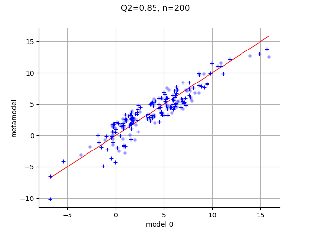
The plot shows that the score is relatively high and might be satisfactory for some purposes. There are however several issues with the previous procedure:

It may happen that the data in the validation sample with size 200 is more difficult to fit than the data in the training dataset. In this case, the $Q^2$ score may be pessimistic.
It may happen that the data in the validation sample with size 200 is less difficult to fit than the data in the validation dataset. In this case, the $Q^2$ score may be optimistic.
We may not be able to generate an extra dataset for validation. In this case, a part of the original dataset should be used for validation.
The polynomial degree may not be appropriate for this data.
The dataset may be ordered in some way, so that the split is somewhat arbitrary. One solution to circumvent this is to randomly shuffle the data. This can be done using the KPermutationsDistribution.

The K-Fold validation aims at solving some of these issues, so that all the available data is used in order to estimate the $Q^2$ score.

In the following script, we compute the $Q^2$ score associated with each polynomial degree from 1 to 10.

degree_max = 10
degree_list = list(range(1, degree_max))
n_degrees = len(degree_list)
score_sample = ot.Sample(len(degree_list), 1)
for i in range(n_degrees):
    totalDegree = degree_list[i]
    score_sample[i, 0] = compute_Q2_score_by_splitting(
        X, Y, basis, totalDegree, im.distributionX
    )
    print(f"split - degree = {totalDegree}, score = {score_sample[i, 0]:.4f}")

split - degree = 1, score = 0.2099
split - degree = 2, score = 0.2400
split - degree = 3, score = 0.4943
split - degree = 4, score = 0.7599
split - degree = 5, score = 0.8438
split - degree = 6, score = 0.9777
split - degree = 7, score = 0.9903
split - degree = 8, score = 0.9996
split - degree = 9, score = 0.9998

graph = ot.Graph("Split", "Degree", "$Q^2$", True)
cloud = ot.Cloud(ot.Sample.BuildFromPoint(degree_list), score_sample)
graph.add(cloud)
view = otv.View(graph)

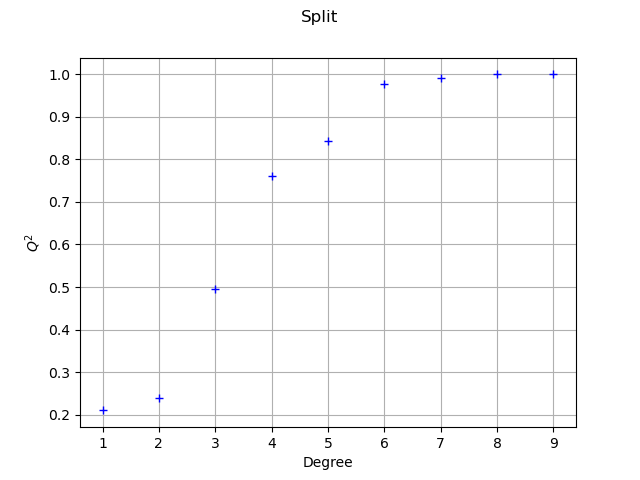
We see that the polynomial degree may be increased up to degree 7, after which the $Q^2$ score does not increase much.

One limitation of the previous method is that the estimate of the $Q^2$ may be sensitive to the particular split of the dataset. The following script uses 5-Fold cross validation to estimate the $Q^2$ score.

score_sample = ot.Sample(len(degree_list), 1)
for i in range(n_degrees):
    totalDegree = degree_list[i]
    score_sample[i, 0] = compute_Q2_score_by_kfold(
        X, Y, basis, totalDegree, im.distributionX
    )
    print(f"k-fold, degree = {totalDegree}, score = {score_sample[i, 0]:.4f}")

k-fold, degree = 1, score = 0.1836
k-fold, degree = 2, score = 0.2017
k-fold, degree = 3, score = 0.4549
k-fold, degree = 4, score = 0.7208
k-fold, degree = 5, score = 0.8423
k-fold, degree = 6, score = 0.9783
k-fold, degree = 7, score = 0.9904
k-fold, degree = 8, score = 0.9996
k-fold, degree = 9, score = 0.9998

graph = ot.Graph("K-Fold", "Degree", "$Q^2$", True)
cloud = ot.Cloud(ot.Sample.BuildFromPoint(degree_list), score_sample)
graph.add(cloud)
view = otv.View(graph)

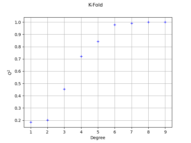
The conclusion is similar to the previous method.

When we select the best polynomial degree which maximizes the $Q^2$ score, the danger is that the validation set is used both for computing the $Q^2$ and to maximize it: hence, the $Q^2$ score may be optimistic. In [muller2016], chapter 5, page 269, the authors advocate the split of the dataset into three subsets:

the training set,
the validation set,
the test set.

When selecting the best parameters, the validation set is used. When estimating the $Q^2$ score with the best parameters, the test set is used.

otv.View.ShowAll()

Total running time of the script: ( 0 minutes 45.118 seconds)

OpenTURNS

An Open source initiative for the Treatment of Uncertainties, Risks'N Statistics

Previous topic

Next topic

This Page

Chaos cross-validation¶