Note
Go to the end to download the full example code
Create a process from random vectors and processes
The objective is to create a process defined from a random vector and a process.
We consider the following limit state function, defined as the difference between a degrading resistance and a time-varying load
:
We propose the following probabilistic model:
- is the initial resistance, and
;
-
is the deterioration rate of the resistance; it is deterministic;
-
is the time-varying stress, which is modeled by a stationary Gaussian process of mean value
, standard deviation
and a squared exponential covariance model;
-
is the time, varying in
.
First, import the python modules:
import openturns as ot
from openturns.viewer import View
import math as m
1. Create the gaussian process  
Create the mesh which is a regular grid on , with
, by step =1:
b = 0.01
t0 = 0.0
step = 1
tfin = 50
n = round((tfin - t0) / step)
myMesh = ot.RegularGrid(t0, step, n)
Create the squared exeponential covariance model:
where the scale parameter is and the amplitude
.
ll = 10 / m.sqrt(2)
myCovKernel = ot.SquaredExponential([ll])
print("cov model = ", myCovKernel)
cov model = SquaredExponential(scale=[7.07107], amplitude=[1])
Create the gaussian process :
S_proc = ot.GaussianProcess(myCovKernel, myMesh)
2. Create the process  
First, create the random variable , with
and
:
muR = 5
sigR = 0.3
R = ot.Normal(muR, sigR)
The create the Dirac random variable :
B = ot.Dirac(b)
Then create the process using the
class and the functional basis
and
:
with independent.
const_func = ot.SymbolicFunction(["t"], ["1"])
linear_func = ot.SymbolicFunction(["t"], ["-t"])
myBasis = ot.Basis([const_func, linear_func])

coef = ot.ComposedDistribution([R, B])

R_proc = ot.FunctionalBasisProcess(coef, myBasis, myMesh)
3. Create the process  
First, aggregate both processes into one process of dimension 2:
myRS_proc = ot.AggregatedProcess([R_proc, S_proc])
Then create the spatial field function that acts only on the values of the process, keeping the mesh unchanged, using the ValueFunction class.
We define the function on
by:
in order to define the spatial field function that acts on fields, defined by:
g = ot.SymbolicFunction(["x1", "x2"], ["x1-x2"])
gDyn = ot.ValueFunction(g, myMesh)
Now you have to create the final process thanks to
:
Z_proc = ot.CompositeProcess(gDyn, myRS_proc)
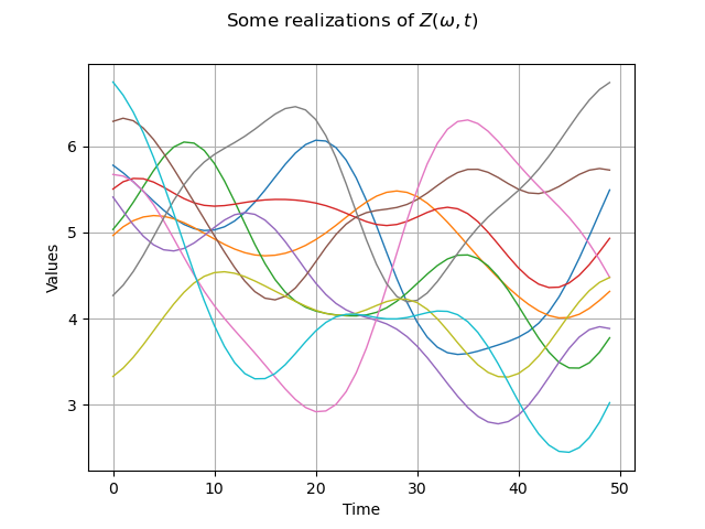
4. Draw some realizations of the process
N = 10
sampleZ_proc = Z_proc.getSample(N)
graph = sampleZ_proc.drawMarginal(0)
graph.setTitle(r"Some realizations of $Z(\omega, t)$")
view = View(graph)

5. Evaluate the probability that  
We define the domaine and the event
:
domain = ot.Interval([2], [4])
print("D = ", domain)
event = ot.ProcessEvent(Z_proc, domain)
D = [2, 4]
We use the Monte Carlo sampling to evaluate the probability:
MC_algo = ot.ProbabilitySimulationAlgorithm(event)
MC_algo.setMaximumOuterSampling(1000000)
MC_algo.setBlockSize(100)
MC_algo.setMaximumCoefficientOfVariation(0.01)
MC_algo.run()

result = MC_algo.getResult()

proba = result.getProbabilityEstimate()
print("Probability = ", proba)
variance = result.getVarianceEstimate()
print("Variance Estimate = ", variance)
IC90_low = proba - result.getConfidenceLength(0.90) / 2
IC90_upp = proba + result.getConfidenceLength(0.90) / 2
print("IC (90%) = [", IC90_low, ", ", IC90_upp, "]")
view.ShowAll()
Probability =  0.7502941176470588
Variance Estimate =  5.565717808041743e-05
IC (90%) = [ 0.7380228946505969 ,  0.7625653406435207 ]
Total running time of the script: ( 0 minutes 0.164 seconds)
 OpenTURNS