Sobol’ sensitivity indices from chaos

In this example we are going to compute global sensitivity indices from a functional chaos decomposition.

We study the Borehole function that models water flow through a borehole:

With parameters:

• : radius of borehole (m)

• : radius of influence (m)

• : transmissivity of upper aquifer ()

• : potentiometric head of upper aquifer (m)

• : transmissivity of lower aquifer ()

• : potentiometric head of lower aquifer (m)

• : length of borehole (m)

• : hydraulic conductivity of borehole ()

import openturns as ot
from operator import itemgetter
import openturns.viewer as viewer
from matplotlib import pylab as plt

ot.Log.Show(ot.Log.NONE)

borehole model

dimension = 8
input_names = ["rw", "r", "Tu", "Hu", "Tl", "Hl", "L", "Kw"]
model = ot.SymbolicFunction(
    input_names, ["(2*pi_*Tu*(Hu-Hl))/(ln(r/rw)*(1+(2*L*Tu)/(ln(r/rw)*rw^2*Kw)+Tu/Tl))"]
)
coll = [
    ot.Normal(0.1, 0.0161812),
    ot.LogNormal(7.71, 1.0056),
    ot.Uniform(63070.0, 115600.0),
    ot.Uniform(990.0, 1110.0),
    ot.Uniform(63.1, 116.0),
    ot.Uniform(700.0, 820.0),
    ot.Uniform(1120.0, 1680.0),
    ot.Uniform(9855.0, 12045.0),
]
distribution = ot.ComposedDistribution(coll)
distribution.setDescription(input_names)

Freeze r, Tu, Tl from model to go faster

selection = [1, 2, 4]
complement = ot.Indices(selection).complement(dimension)
distribution = distribution.getMarginal(complement)
model = ot.ParametricFunction(
    model, selection, distribution.getMarginal(selection).getMean()
)
input_names_copy = list(input_names)
input_names = itemgetter(*complement)(input_names)
dimension = len(complement)

design of experiment

size = 1000
X = distribution.getSample(size)
Y = model(X)

create a functional chaos model

algo = ot.FunctionalChaosAlgorithm(X, Y)
algo.run()
result = algo.getResult()
print(result.getResiduals())
print(result.getRelativeErrors())

[0.000746196]
[1.4036e-09]

Quick summary of sensitivity analysis

sensitivityAnalysis = ot.FunctionalChaosSobolIndices(result)
print(sensitivityAnalysis)

 input dimension: 5
 output dimension: 1
 basis size: 72
 mean: [74.7248]
 std-dev: [29.4227]
------------------------------------------------------------
Index   | Multi-indice                  | Part of variance
------------------------------------------------------------
      1 | [1,0,0,0,0]                   | 0.662144
      3 | [0,0,1,0,0]                   | 0.0921578
      2 | [0,1,0,0,0]                   | 0.0919831
      4 | [0,0,0,1,0]                   | 0.0879504
      5 | [0,0,0,0,1]                   | 0.0214526
------------------------------------------------------------


------------------------------------------------------------
Component | Sobol index            | Sobol total index
------------------------------------------------------------
        0 | 0.671023               | 0.702031
        1 | 0.0919831              | 0.103275
        2 | 0.0921578              | 0.103503
        3 | 0.0889172              | 0.101317
        4 | 0.0214526              | 0.0247002
------------------------------------------------------------

draw Sobol’ indices

first_order = [sensitivityAnalysis.getSobolIndex(i) for i in range(dimension)]
total_order = [sensitivityAnalysis.getSobolTotalIndex(i) for i in range(dimension)]
graph = ot.SobolIndicesAlgorithm.DrawSobolIndices(input_names, first_order, total_order)
view = viewer.View(graph)

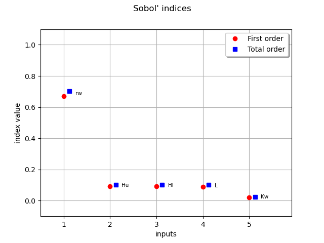
We saw that total order indices are close to first order, so the higher order indices must be all quite close to 0

for i in range(dimension):
    for j in range(i):
        print(
            input_names[i] + " & " + input_names[j],
            ":",
            sensitivityAnalysis.getSobolIndex([i, j]),
        )

plt.show()

Hu & rw : 0.009554440399548765
Hl & rw : 0.009605011708530762
Hl & Hu : 0.0
L & rw : 0.009256817002544384
L & Hu : 0.0012699291331901821
L & Hl : 0.0012715335256775347
Kw & rw : 0.0022389601978756737
Kw & Hu : 0.0003031973629515978
Kw & Hl : 0.00030390360173584134
Kw & L : 0.00030193154550350816