Note
Go to the end to download the full example code
Taylor approximations
In this example we build a local approximation of a model using the
Taylor decomposition using the LinearTaylor class.
We consider the function defined by:
for any .
The metamodel
is is an approximation of the model
:
for any .
In this example, we consider two different approximations:
the first order Taylor expansion,
the second order Taylor expansion.
import openturns as ot
import openturns.viewer as viewer
from matplotlib import pylab as plt

ot.Log.Show(ot.Log.NONE)
Define the model
Prepare some data.
formulas = ["cos(x1 + x2)", "(x2 + 1) * exp(x1 - 2 * x2)"]
model = ot.SymbolicFunction(["x1", "x2"], formulas)
Center of the approximation.
x0 = [-0.4, -0.4]
Drawing bounds.
a = -0.4
b = 0.0
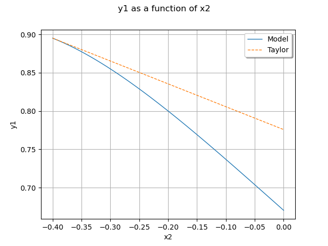
First order Taylor expansion
Let be a reference point where
the linear approximation is evaluated.
The first order Taylor expansion is:
for any .
Create a linear (first-order) Taylor approximation.
algo = ot.LinearTaylor(x0, model)
algo.run()
responseSurface = algo.getMetaModel()
Plot the second output of our model with .
graph = ot.ParametricFunction(model, [0], [x0[1]]).getMarginal(1).draw(a, b)
graph.setLegends(["Model"])
curve = (
    ot.ParametricFunction(responseSurface, [0], [x0[1]]).getMarginal(1).draw(a, b).getDrawable(0)
)
curve.setLegend("Taylor")
curve.setLineStyle("dashed")
graph.add(curve)
graph.setLegendPosition("topright")
graph.setColors(ot.Drawable.BuildDefaultPalette(2))
view = viewer.View(graph)

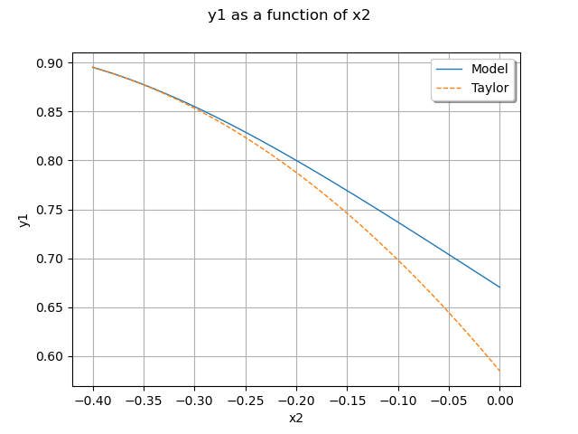
Second order Taylor expansion
Let be a reference point where
the quadratic approximation is evaluated.
The second order Taylor expansion is:
for any .
Create a quadratic (second-order) Taylor approximation.
algo = ot.QuadraticTaylor(x0, model)
algo.run()
responseSurface = algo.getMetaModel()
Plot second output of our model with .
graph = ot.ParametricFunction(model, [0], [x0[1]]).getMarginal(1).draw(a, b)
graph.setLegends(["Model"])
curve = (
    ot.ParametricFunction(responseSurface, [0], [x0[1]]).getMarginal(1).draw(a, b).getDrawable(0)
)
curve.setLegend("Taylor")
curve.setLineStyle("dashed")
graph.add(curve)
graph.setLegendPosition("topright")
graph.setColors(ot.Drawable.BuildDefaultPalette(2))
view = viewer.View(graph)
plt.show()

 OpenTURNS