Estimate moments from Taylor expansions

In this example we are going to estimate mean and standard deviation of an output variable of interest thanks to the Taylor variance decomposition method of order 1 or 2.

Model definition

import openturns as ot
import openturns.viewer as viewer
import numpy as np
from matplotlib import pylab as plt

ot.Log.Show(ot.Log.NONE)

Create a composite random vector

ot.RandomGenerator.SetSeed(0)
input_names = ["x1", "x2", "x3", "x4"]
myFunc = ot.SymbolicFunction(input_names, ["cos(x2*x2+x4)/(x1*x1+1+x3^4)"])
R = ot.CorrelationMatrix(4)
for i in range(4):
    R[i, i - 1] = 0.25
distribution = ot.Normal([0.2] * 4, [0.1, 0.2, 0.3, 0.4], R)
distribution.setDescription(input_names)
# We create a distribution-based RandomVector
X = ot.RandomVector(distribution)
# We create a composite RandomVector Y from X and myFunc
Y = ot.CompositeRandomVector(myFunc, X)

Taylor expansion based estimation of the moments

We create a Taylor expansion method to approximate moments

taylor = ot.TaylorExpansionMoments(Y)

Analysis of the results

get 1st order mean

print(taylor.getMeanFirstOrder())

[0.932544]

get 2nd order mean

print(taylor.getMeanSecondOrder())

[0.820295]

get covariance

print(taylor.getCovariance())

[[ 0.0124546 ]]

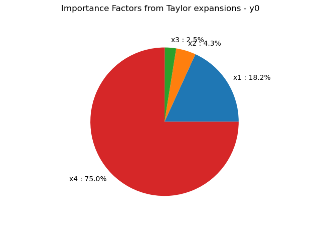
draw importance factors

taylor.getImportanceFactors()

[x1 : 0.181718, x2 : 0.0430356, x3 : 0.0248297, x4 : 0.750417]

draw importance factors

graph = taylor.drawImportanceFactors()
view = viewer.View(graph)

Get the value of the output at the mean point

taylor.getValueAtMean()

[0.932544]

Get the gradient value of the output at the mean point

taylor.getGradientAtMean()

[[ -0.35812 ]
[ -0.0912837 ]
[ -0.0286496 ]
[ -0.228209 ]]

Get the hessian value of the output at the mean point

taylor.getHessianAtMean()
plt.show()

Using finite difference gradients

When no gradient and/or functions are provided for the model, a finite difference approach is relied on automatically. However, it is possible to manually specify the characteristic of the considered difference steps.

def myPythonFunction(X):
    x1, x2, x3, x4 = X
    return [np.cos(x2 * x2 + x4) / (x1 * x1 + 1.0 + x3 ** 4)]


myFunc = ot.PythonFunction(4, 1, myPythonFunction)

For instance, a user-defined constant step value can be considered

gradEpsilon = [1e-8] * 4
hessianEpsilon = [1e-7] * 4
gradStep = ot.ConstantStep(gradEpsilon)  # Costant gradient step
hessianStep = ot.ConstantStep(hessianEpsilon)  # Constant Hessian step
myFunc.setGradient(
    ot.CenteredFiniteDifferenceGradient(gradStep, myFunc.getEvaluation())
)
myFunc.setHessian(
    ot.CenteredFiniteDifferenceHessian(hessianStep, myFunc.getEvaluation())
)

Alternatively, we can consider a finite difference step value which depends on the location in the input space by relying on the BlendedStep class:

gradEpsilon = [1e-8] * 4
hessianEpsilon = [1e-7] * 4
gradStep = ot.BlendedStep(gradEpsilon)  # Costant gradient step
hessianStep = ot.BlendedStep(hessianEpsilon)  # Constant Hessian step
myFunc.setGradient(
    ot.CenteredFiniteDifferenceGradient(gradStep, myFunc.getEvaluation())
)
myFunc.setHessian(
    ot.CenteredFiniteDifferenceHessian(hessianStep, myFunc.getEvaluation())
)

We can then proceed in the same way as before

Y = ot.CompositeRandomVector(myFunc, X)
taylor = ot.TaylorExpansionMoments(Y)