 OpenTURNS
Note
Go to the end to download the full example code.
Select fitted copulas
In this example we select the copula which best fits a sample. It mirrors Select fitted distributions, which deals with the marginal distributions, but focuses here on the dependence structure.
Two complementary tools are combined:
ranking by BIC values with
BestModelBIC(),ranking by the p-values of the copula goodness-of-fit tests (
CopulaCramerVonMises()andCopulaKolmogorov(), see Goodness-of-fit tests for copulas).
The normalization step required before computing a BIC on a copula is described in detail below.
import openturns as ot
import openturns.viewer as otv

ot.RandomGenerator.SetSeed(1)
Create data with a known dependence structure
We sample a joint distribution with non-uniform marginals and a Gumbel copula,
as is typical of real observations: the sample does not live in  .
true_copula = ot.GumbelCopula(4.0)
marginals = [ot.Normal(), ot.Exponential()]
distribution = ot.JointDistribution(marginals, true_copula)
size = 500
sample = distribution.getSample(size)
print("sample min/max=", sample.getMin(), sample.getMax())
sample min/max= [-3.4174,0.000155593] [2.8932,6.37817]
1. Rank copulas by BIC
A copula is a distribution on : its probability density
function is zero outside the unit hypercube. The BIC evaluates the
log-likelihood of the sample under each candidate, so it must be computed
on points inside . Applied to the raw observations, it
saturates to infinity:
copula_factories = [
    ot.GumbelCopulaFactory(),
    ot.ClaytonCopulaFactory(),
    ot.NormalCopulaFactory(),
    ot.FrankCopulaFactory(),
    ot.IndependentCopulaFactory(),
]
for factory in copula_factories:
    _, bic = ot.FittingTest.BIC(sample, factory)
    print(f"{factory.getClassName():25s} BIC={bic:.3f}")
GumbelCopulaFactory       BIC=inf
ClaytonCopulaFactory      BIC=inf
NormalCopulaFactory       BIC=inf
FrankCopulaFactory        BIC=inf
IndependentCopulaFactory  BIC=inf
Note that a simple min/max rescaling to is not sufficient:
the boundary points then sit exactly on the border of the support, where the
log-PDF of most copulas is still degenerated, and the rescaled margins are
not uniform anyway. The sample must instead be mapped to uniform margins
while preserving the dependence structure. The standard rank-based mapping
uses the pseudo-observations  , where
 is the rank of
 within its margin:
pseudo_sample = (sample.rank() + 1.0) / (size + 1.0)
print("pseudo min/max=", pseudo_sample.getMin(), pseudo_sample.getMax())
pseudo min/max= [0.00199601,0.00199601] [0.998004,0.998004]
An alternative, used in Estimate a multivariate distribution, maps each margin through its fitted cumulative distribution function. Both mappings coincide asymptotically; ranks need no marginal estimation.
The BIC ranking is then meaningful and selects the true family:
for factory in copula_factories:
    _, bic = ot.FittingTest.BIC(pseudo_sample, factory)
    print(f"{factory.getClassName():25s} BIC={bic:.3f}")
best_copula, best_bic = ot.FittingTest.BestModelBIC(pseudo_sample, copula_factories)
print("best copula:", best_copula)
print("best BIC:", best_bic)
GumbelCopulaFactory       BIC=-2.106
ClaytonCopulaFactory      BIC=-1.148
NormalCopulaFactory       BIC=-2.041
FrankCopulaFactory        BIC=-1.848
IndependentCopulaFactory  BIC=0.000
best copula: GumbelCopula(theta = 4.31452)
best BIC: -2.10610538747555
The same holds with fully specified copulas instead of factories:
candidates = [ot.GumbelCopula(4.0), ot.ClaytonCopula(6.0), ot.FrankCopula(5.0)]
for copula in candidates:
    bic = ot.FittingTest.BIC(pseudo_sample, copula)
    print(f"{copula.getClassName():15s} BIC={bic:.3f}")
GumbelCopula    BIC=-2.109
ClaytonCopula   BIC=-1.281
FrankCopula     BIC=-1.166
2. Rank copulas by goodness-of-fit tests
Unlike the BIC, the copula Cramer-von Mises and Kolmogorov tests of Goodness-of-fit tests for copulas are rank-based: the pseudo-observations are computed internally, so the tests apply directly to the raw observations. With a factory, the copula parameters are estimated from the sample and the p-value is computed by parametric bootstrap:
Reduce the bootstrap cost for the documentation; use the default ResourceMap keys for real studies.
ot.ResourceMap.SetAsUnsignedInteger("FittingTest-CopulaMinimumSamplingSize", 10)
ot.ResourceMap.SetAsUnsignedInteger("FittingTest-CopulaMaximumSamplingSize", 100)
for factory in [ot.GumbelCopulaFactory(), ot.ClaytonCopulaFactory()]:
    estimated, result = ot.FittingTest.CopulaCramerVonMises(sample, factory)
    print(
        f"{factory.getClassName():25s} p-value={result.getPValue():.3f} "
        f"statistic={result.getStatistic():.4f} "
        f"accept={result.getBinaryQualityMeasure()} estimated={estimated}"
    )
ot.ResourceMap.Reset()
GumbelCopulaFactory       p-value=0.260 statistic=0.0131 accept=True estimated=GumbelCopula(theta = 4.31452)
ClaytonCopulaFactory      p-value=0.000 statistic=0.1702 accept=False estimated=ClaytonCopula(theta = 6.62904)
The Kolmogorov variant behaves similarly; here on the best BIC candidate:
ot.ResourceMap.SetAsUnsignedInteger("FittingTest-CopulaMaximumSamplingSize", 100)
estimated, result = ot.FittingTest.CopulaKolmogorov(sample, ot.GumbelCopulaFactory())
print("estimated:", estimated)
print(result)
ot.ResourceMap.Reset()
estimated: GumbelCopula(theta = 4.31452)
class=TestResult name=Unnamed type=CopulaKolmogorov GumbelCopula binaryQualityMeasure=true p-value threshold=0.05 p-value=0.27 statistic=0.0169293 description=[GumbelCopula(theta = 4.31452) vs sample JointDistribution]
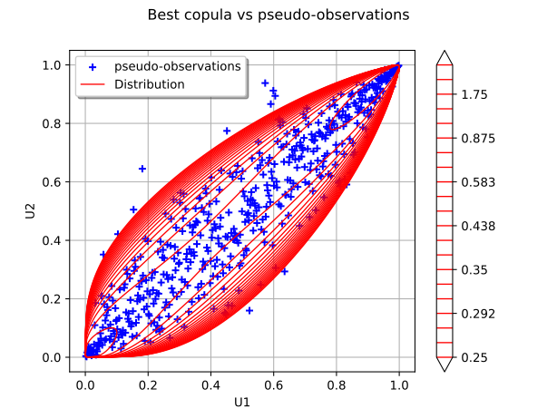
Graphical validation in the rank space
We plot the pseudo-observations with the iso-curves of the selected copula, as in Test the copula:
cloud = ot.Cloud(pseudo_sample, "blue", "plus", "pseudo-observations")
graph = ot.Graph("Best copula vs pseudo-observations", "U1", "U2")
graph.add(cloud)
pdf_graph = best_copula.drawPDF([0.0] * 2, [1.0] * 2, [201] * 2)
contour = pdf_graph.getDrawable(0)
contour.setDrawLabels(False)
nlev = 21
contour.setLevels([0.25 * nlev / (nlev - i) for i in range(nlev)])
contour.setLegend(str(best_copula.getClassName()))
contour.setColor("red")
graph.add(contour)
graph.setLegendPosition("upper left")
view = otv.View(graph)
otv.View.ShowAll()