Kriging: choose a polynomial trend on the beam model

The goal of this example is to show how to configure the trend in a Kriging metamodel. This example focuses on three polynomial trends:

• ConstantBasisFactory,

• LinearBasisFactory,

• QuadraticBasisFactory.

In the Kriging: choose a polynomial trend example, we give another example of this procedure.

For this purpose, we use the cantilever beam example.

Definition of the model

from openturns.usecases import cantilever_beam
import openturns as ot
from openturns.viewer import View

ot.RandomGenerator.SetSeed(0)
ot.Log.Show(ot.Log.NONE)

We load the use case :

cb = cantilever_beam.CantileverBeam()

We define the function which evaluates the output depending on the inputs.

model = cb.model

Then we define the distribution of the input random vector.

dimension = cb.dim  # number of inputs
myDistribution = cb.distribution

Create the design of experiments

We consider a simple Monte-Carlo sampling as a design of experiments. This is why we generate an input sample using the getSample() method of the distribution. Then we evaluate the output using the model function.

sampleSize_train = 10
X_train = myDistribution.getSample(sampleSize_train)
Y_train = model(X_train)

Create the metamodel

In order to create the Kriging metamodel, we first select a constant trend with the ConstantBasisFactory class. Then we use a squared exponential covariance kernel. The SquaredExponential kernel has one amplitude coefficient and 4 scale coefficients. This is because this covariance kernel is anisotropic : each of the 4 input variables is associated with its own scale coefficient.

basis = ot.ConstantBasisFactory(dimension).build()
covarianceModel = ot.SquaredExponential(dimension)

Typically, the optimization algorithm is quite good at setting sensible optimization bounds. In this case, however, the range of the input domain is extreme.

print("Lower and upper bounds of X_train:")
print(X_train.getMin(), X_train.getMax())

Lower and upper bounds of X_train:
[6.50185e+10,262.654,2.50948,1.40294e-07] [6.88439e+10,323.088,2.59143,1.5807e-07]

We need to manually define sensible optimization bounds. Note that since the amplitude parameter is computed analytically (this is possible when the output dimension is 1), we only need to set bounds on the scale parameter.

scaleOptimizationBounds = ot.Interval(
    [1.0, 1.0, 1.0, 1.0e-10], [1.0e11, 1.0e3, 1.0e1, 1.0e-5]
)

Finally, we use the KrigingAlgorithm class to create the Kriging metamodel. It requires a training sample, a covariance kernel and a trend basis as input arguments. We need to set the initial scale parameter for the optimization. The upper bound of the input domain is a sensible choice here. We must not forget to actually set the optimization bounds defined above.

covarianceModel.setScale(X_train.getMax())
algo = ot.KrigingAlgorithm(X_train, Y_train, covarianceModel, basis)
algo.setOptimizationBounds(scaleOptimizationBounds)

Run the algorithm and get the result.

algo.run()
result = algo.getResult()
krigingWithConstantTrend = result.getMetaModel()

The getTrendCoefficients method returns the coefficients of the trend.

print(result.getTrendCoefficients())

[0.108219]

The constant trend always has only one coefficient (if there is one single output).

print(result.getCovarianceModel())

SquaredExponential(scale=[6.88439e+10,323.088,2.59143,1.5807e-07], amplitude=[0.247034])

Setting the trend

covarianceModel.setScale(X_train.getMax())
basis = ot.LinearBasisFactory(dimension).build()
algo = ot.KrigingAlgorithm(X_train, Y_train, covarianceModel, basis)
algo.setOptimizationBounds(scaleOptimizationBounds)
algo.run()
result = algo.getResult()
krigingWithLinearTrend = result.getMetaModel()
result.getTrendCoefficients()

class=Point name=Unnamed dimension=5 values=[-8.81529e-25,-1.00576e-13,-2.65632e-22,-2.22154e-24,-1.3279e-31]

The number of coefficients in the linear and quadratic trends depends on the number of inputs, which is equal to

in the cantilever beam case.

We observe that the number of coefficients in the trend is 5, which corresponds to:

• 1 coefficient for the constant part,

• dim=4 coefficients for the linear part.

covarianceModel.setScale(X_train.getMax())
basis = ot.QuadraticBasisFactory(dimension).build()
algo = ot.KrigingAlgorithm(X_train, Y_train, covarianceModel, basis)
algo.setOptimizationBounds(scaleOptimizationBounds)
algo.run()
result = algo.getResult()
krigingWithQuadraticTrend = result.getMetaModel()
result.getTrendCoefficients()
print(algo.getOptimizationBounds())
print(result.getCovarianceModel())

[1, 1e+11]
[1, 1000]
[1, 10]
[1e-10, 1e-05]
SquaredExponential(scale=[6.88439e+10,323.088,2.59143,1.5807e-07], amplitude=[1.74417e-10])

This time, the trend has 15 coefficients:

• 1 coefficient for the constant part,

• 4 coefficients for the linear part,

• 10 coefficients for the quadratic part.

This is because the number of coefficients in the quadratic part has

coefficients, associated with the symmetric matrix of the quadratic function.

Validate the metamodel

We finally want to validate the Kriging metamodel. This is why we generate a validation sample with size 100 and we evaluate the output of the model on this sample.

sampleSize_test = 100
X_test = myDistribution.getSample(sampleSize_test)
Y_test = model(X_test)

def drawMetaModelValidation(X_test, Y_test, krigingMetamodel, title):
    val = ot.MetaModelValidation(Y_test, krigingMetamodel(X_test))
    R2 = val.computeR2Score()[0]
    graph = val.drawValidation().getGraph(0, 0)
    graph.setLegends([""])
    graph.setLegends(["%s, R2 = %.2f%%" % (title, 100 * R2), ""])
    graph.setLegendPosition("upper left")
    return graph

grid = ot.GridLayout(1, 3)
grid.setTitle("Different trends")
graphConstant = drawMetaModelValidation(
    X_test, Y_test, krigingWithConstantTrend, "Constant"
)
graphLinear = drawMetaModelValidation(X_test, Y_test, krigingWithLinearTrend, "Linear")
graphQuadratic = drawMetaModelValidation(
    X_test, Y_test, krigingWithQuadraticTrend, "Quadratic"
)
grid.setGraph(0, 0, graphConstant)
grid.setGraph(0, 1, graphLinear)
grid.setGraph(0, 2, graphQuadratic)
_ = View(grid, figure_kw={"figsize": (13, 4)})

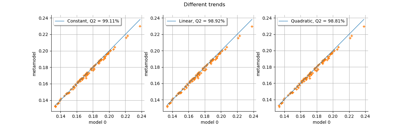
We observe that the three trends perform very well in this case. With more coefficients, the Kriging metamodel is more flexibile and can adjust better to the training sample. This does not mean, however, that the trend coefficients will provide a good fit for the validation sample.

The number of parameters in each Kriging metamodel is the following:

• the constant trend Kriging has 6 coefficients to estimate: 5 coefficients for the covariance matrix and 1 coefficient for the trend,

• the linear trend Kriging has 10 coefficients to estimate: 5 coefficients for the covariance matrix and 5 coefficients for the trend,

• the quadratic trend Kriging has 20 coefficients to estimate: 5 coefficients for the covariance matrix and 15 coefficients for the trend.

In the cantilever beam example, fitting the metamodel to a training sample with only 10 points is made much easier because the function to approximate is almost linear. In this case, a quadratic trend is not advisable because it can interpolate all points in the training sample.