Note
Go to the end to download the full example code.
Kriging with an isotropic covariance function
In typical machine learning applications, Gaussian process regression/Kriging surrogate models take several inputs, and those inputs are usually heterogeneous (e.g. in the cantilever beam use case, inputs are various physical quantities).
In geostatistical applications however, inputs are typically spatial
coordinates, which means one can assume the output varies at the same rate
in all directions.
This calls for a specific kind of covariance kernel, represented
in the library by the IsotropicCovarianceModel class.
Modeling temperature across a surface
In this example, we collect temperature data over a floorplan using sensors.
import numpy as np
import openturns as ot
import matplotlib.pyplot as plt

ot.Log.Show(ot.Log.NONE)

coordinates = ot.Sample(
    [
        [100.0, 100.0],
        [500.0, 100.0],
        [900.0, 100.0],
        [100.0, 350.0],
        [500.0, 350.0],
        [900.0, 350.0],
        [100.0, 600.0],
        [500.0, 600.0],
        [900.0, 600.0],
    ]
)
observations = ot.Sample(
    [[25.0], [25.0], [10.0], [20.0], [25.0], [20.0], [15.0], [25.0], [25.0]]
)
Let us plot the data.
# Extract coordinates.
x = np.array(coordinates[:, 0])
y = np.array(coordinates[:, 1])

# Plot the data with a scatter plot and a color map.
fig = plt.figure()
plt.scatter(x, y, c=observations, cmap="viridis")
plt.colorbar()
plt.show()

Because we are going to view several Kriging models in this example,
we use a function to automate the process of optimizing the scale parameter
and producing the metamodel.
Since version 1.15 of the library, input data are no longer rescaled by the
KrigingAlgorithm class, so we need to manually set
sensible bounds for the scale parameter.
lower = 50.0
upper = 1000.0


def fitKriging(coordinates, observations, covarianceModel, basis):
    """
    Fit the parameters of a Kriging metamodel.
    """
    # Define the Kriging algorithm.
    algo = ot.KrigingAlgorithm(coordinates, observations, covarianceModel, basis)

    # Set the optimization bounds for the scale parameter to sensible values
    # given the data set.
    scale_dimension = covarianceModel.getScale().getDimension()
    algo.setOptimizationBounds(
        ot.Interval([lower] * scale_dimension, [upper] * scale_dimension)
    )

    # Run the Kriging algorithm and extract the fitted surrogate model.
    algo.run()
    krigingResult = algo.getResult()
    krigingMetamodel = krigingResult.getMetaModel()
    return krigingResult, krigingMetamodel
Let us define a helper function to plot Kriging predictions.
def plotKrigingPredictions(krigingMetamodel):
    """
    Plot the predictions of a Kriging metamodel.
    """
    # Create the mesh of the box [0., 1000.] * [0., 700.]
    myInterval = ot.Interval([0.0, 0.0], [1000.0, 700.0])

    # Define the number of intervals in each direction of the box
    nx = 20
    ny = 20
    myIndices = [nx - 1, ny - 1]
    myMesher = ot.IntervalMesher(myIndices)
    myMeshBox = myMesher.build(myInterval)

    # Predict
    vertices = myMeshBox.getVertices()
    predictions = krigingMetamodel(vertices)

    # Format for plot
    X = np.array(vertices[:, 0]).reshape((ny, nx))
    Y = np.array(vertices[:, 1]).reshape((ny, nx))
    predictions_array = np.array(predictions).reshape((ny, nx))

    # Plot
    plt.figure()
    plt.pcolormesh(X, Y, predictions_array, shading="auto")
    plt.colorbar()
    plt.show()
    return
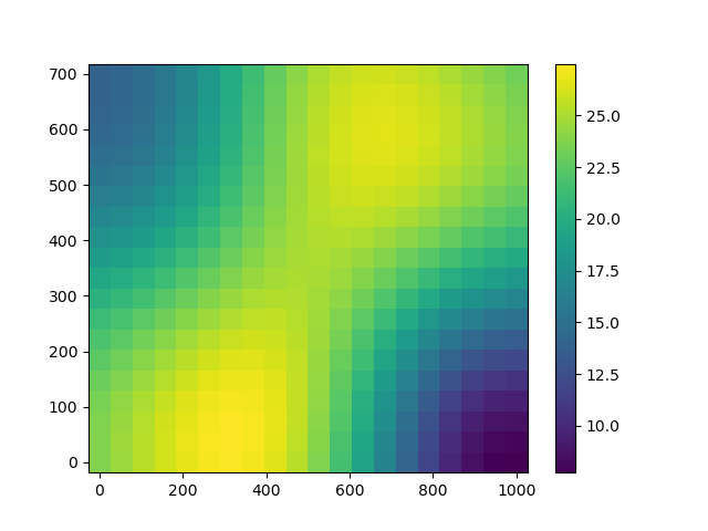
Predict with an anisotropic geometric covariance kernel
In order to illustrate the usefulness of isotropic covariance kernels, we first perform prediction with an anisotropic geometric kernel.
Keep in mind that, when there are more than one input dimension,
the CovarianceModel classes use a multidimensional
scale parameter  .
They are anisotropic geometric by default.
.
They are anisotropic geometric by default.
Our example has two input dimensions,
so  .
.
inputDimension = 2
basis = ot.ConstantBasisFactory(inputDimension).build()
covarianceModel = ot.SquaredExponential(inputDimension)
krigingResult, krigingMetamodel = fitKriging(
    coordinates, observations, covarianceModel, basis
)
plotKrigingPredictions(krigingMetamodel)
We see weird vertical columns on the plot.
How did this happen? Let us have a look at the optimized scale parameter
 .
.
print(krigingResult.getCovarianceModel().getScale())
[50,344.874]
The value of  is actually equal to the lower bound:
print(lower)
50.0
This means that temperatures are likely to vary a lot along the X axis and much slower across the Y axis based on the observation data.
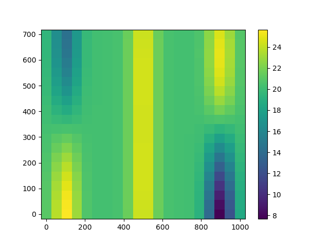
Predict with an isotropic covariance kernel
If we know that variations of the temperature are isotropic (i.e. with no priviledged direction), we can embed this information within the covariance kernel.
isotropic = ot.IsotropicCovarianceModel(ot.SquaredExponential(), inputDimension)
The IsotropicCovarianceModel class creates an isotropic
version with a given input dimension of a CovarianceModel.
Because is is isotropic, it only needs one scale parameter  and it will make sure
  at all times
during the optimization.
at all times
during the optimization.
krigingResult, krigingMetamodel = fitKriging(
    coordinates, observations, isotropic, basis
)
print(krigingResult.getCovarianceModel().getScale())
[286.426]
Prediction with the isotropic covariance kernel is much more satisfactory.
# sphinx_gallery_thumbnail_number = 3
plotKrigingPredictions(krigingMetamodel)