Kriging: propagate uncertainties

In this example we propagate uncertainties through a Kriging metamodel of the Ishigami model.

import openturns as ot
from matplotlib import pylab as plt
import openturns.viewer as otv

We first build the metamodel and then compute its mean with a Monte-Carlo computation.

We load the Ishigami model from the usecases module:

from openturns.usecases import ishigami_function

im = ishigami_function.IshigamiModel()

We build a design of experiments with a Latin Hypercube Sampling (LHS) for the three input variables supposed independent.

experiment = ot.LHSExperiment(im.inputDistribution, 30, False, True)
xdata = experiment.generate()

We get the exact model and evaluate it at the input training data xdata to build the output data ydata.

model = im.model
ydata = model(xdata)

We define our Kriging strategy :

• a constant basis in ;

• a squared exponential covariance function.

dimension = 3
basis = ot.ConstantBasisFactory(dimension).build()
covarianceModel = ot.SquaredExponential([0.1] * dimension, [1.0])
algo = ot.KrigingAlgorithm(xdata, ydata, covarianceModel, basis)
algo.run()
result = algo.getResult()

We finally get the metamodel to use with Monte-Carlo.

metamodel = result.getMetaModel()

We want to estmate the mean of the Ishigami model with Monte-Carlo using the metamodel instead of the exact model.

We first create a random vector following the input distribution :

X = ot.RandomVector(im.inputDistribution)

And then we create a random vector from the image of the input random vector by the metamodel :

Y = ot.CompositeRandomVector(metamodel, X)

We now set our ExpectationSimulationAlgorithm object :

algo = ot.ExpectationSimulationAlgorithm(Y)
algo.setMaximumOuterSampling(50000)
algo.setBlockSize(1)
algo.setCoefficientOfVariationCriterionType("NONE")

We run it and store the results :

algo.run()
result = algo.getResult()

The expectation ( mean ) is obtained with :

expectation = result.getExpectationEstimate()

The mean estimate of the metamodel is

print("Mean of the Ishigami metamodel : %.3e" % expectation[0])

Mean of the Ishigami metamodel : 3.065e+00

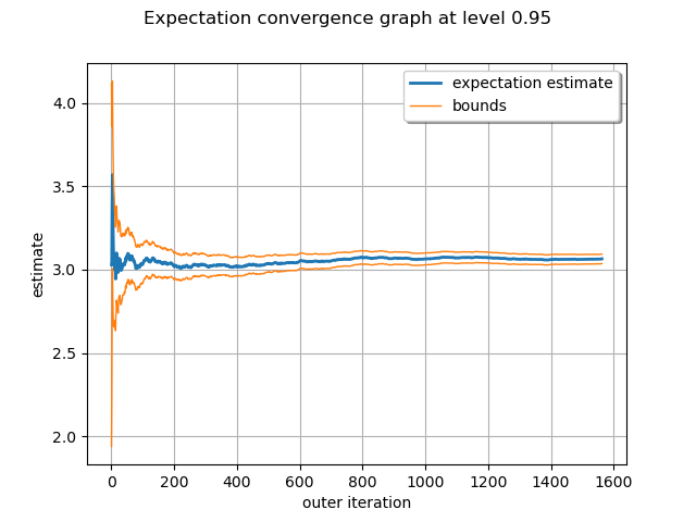
We draw the convergence history.

graph = algo.drawExpectationConvergence()
view = otv.View(graph)

For reference, the exact mean of the Ishigami model is :

print("Mean of the Ishigami model : %.3e" % im.expectation)

plt.show()

Mean of the Ishigami model : 3.500e+00