Introduction to OpenTURNS objects

In the otbenchmark package, we use several objects that must be known in order to distinguish which objects come from the OpenTURNS library or from otbenchmark. For reliability problems, there are three objects that cannot be ignored:

• the openturns.Distribution,

• the openturns.Function,

• the openturns.ThresholdEvent.

import openturns as ot
import matplotlib.pyplot as plt
import openturns.viewer as otv

Avoid mixture warnings

ot.Log.Show(ot.Log.NONE)

Distribution

Define two marginals

X0 = ot.Normal(0.0, 1.0)
X1 = ot.Uniform(0.0, 1.0)

Define an independent joint distribution

X_ind = ot.ComposedDistribution([X0, X1])

Define a dependent joint distribution using a copula (e.g., Frank copula)

copula = ot.FrankCopula(5)
X_dep = ot.ComposedDistribution([X0, X1], copula)

Generate a sample of each joint distribution

X_ind_sample = X_ind.getSample(1000)
X_dep_sample = X_dep.getSample(1000)

method_list = [method for method in dir(X0) if method.startswith("__") is False]
print(len(method_list))

145

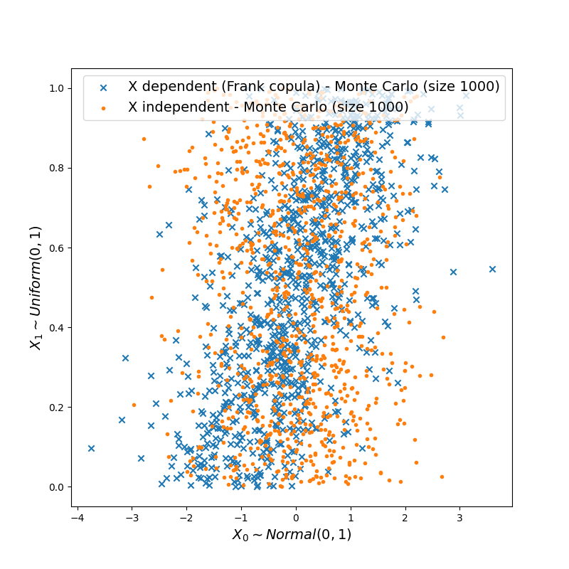
plt.figure(figsize=(8, 8))
plt.scatter(
    X_dep_sample[:, 0],
    X_dep_sample[:, 1],
    label="X dependent (Frank copula) - Monte Carlo (size 1000)",
    marker="x",
)
plt.scatter(
    X_ind_sample[:, 0],
    X_ind_sample[:, 1],
    label="X independent - Monte Carlo (size 1000)",
    marker=".",
)

plt.xlabel(r"$X_0 \sim Normal(0, 1)$", fontsize=14)
plt.ylabel(r"$X_1 \sim Uniform(0, 1)$", fontsize=14)
_ = plt.legend(loc="best", fontsize=14)

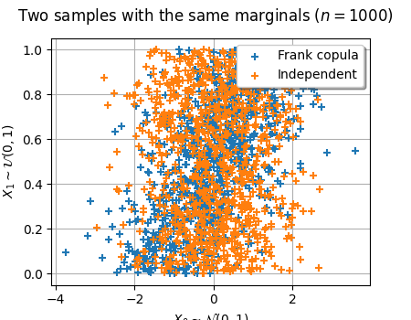
graph = ot.Graph(
    "Two samples with the same marginals ($n=1000$)",
    r"$X_0 \sim \mathcal{N}(0, 1)$",
    r"$X_1 \sim \mathcal{U}(0, 1)$",
    True,
)
cloud = ot.Cloud(X_dep_sample[:, 0], X_dep_sample[:, 1])
cloud.setLegend("Frank copula")
graph.add(cloud)
cloud = ot.Cloud(X_ind_sample[:, 0], X_ind_sample[:, 1])
cloud.setLegend("Independent")
graph.add(cloud)
graph.setLegendPosition("topright")
graph.setColors(ot.Drawable.BuildDefaultPalette(2))
view = otv.View(graph, figure_kw={"figsize": (4.5, 3.5)})
# view.save("two_samples.pdf")

Function

Define a symbolic function

myfunction = ot.SymbolicFunction(["x0", "x1"], ["sin(x0) * (1 + x1 ^ 2)"])
myfunction.setInputDescription(["$x_0$", "$x_1$"])
myfunction.setOutputDescription(["$y$"])

Define input random vectors

inputVect_ind = ot.RandomVector(X_ind)
inputVect_dep = ot.RandomVector(X_dep)

Compose input random vectors by the symbolic function

outputVect_ind = ot.CompositeRandomVector(myfunction, inputVect_ind)
outputVect_dep = ot.CompositeRandomVector(myfunction, inputVect_dep)

Sample the output random variable

outputSample_ind = outputVect_ind.getSample(10000)
outputSample_dep = outputVect_dep.getSample(10000)

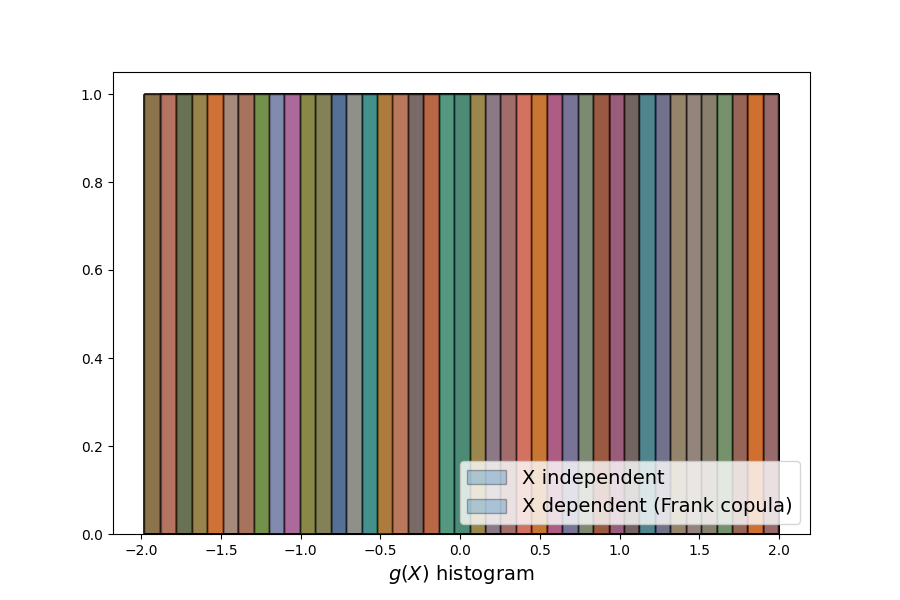
plt.figure(figsize=(9, 6))
plt.hist(
    outputSample_ind,
    bins=40,
    histtype="stepfilled",
    alpha=0.3,
    ec="k",
    label="X independent",
)
plt.hist(
    outputSample_dep,
    bins=40,
    histtype="stepfilled",
    alpha=0.3,
    ec="k",
    label="X dependent (Frank copula)",
)
plt.xlabel("$g(X)$ histogram", fontsize=14)
_ = plt.legend(loc="best", fontsize=14)

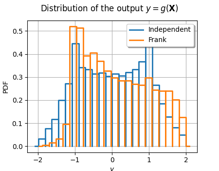
graph = ot.HistogramFactory().build(outputSample_ind).drawPDF()
graph.setLegends(["Independent"])
graph.setTitle(r"Distribution of the output $y=g(\mathbf{X})$")
curve = ot.HistogramFactory().build(outputSample_dep).drawPDF()
curve.setLegends(["Frank"])
graph.add(curve)
graph.setColors(ot.Drawable.BuildDefaultPalette(2))
view = otv.View(graph, figure_kw={"figsize": (4.5, 3.5)})
# view.save("histo_output.pdf")

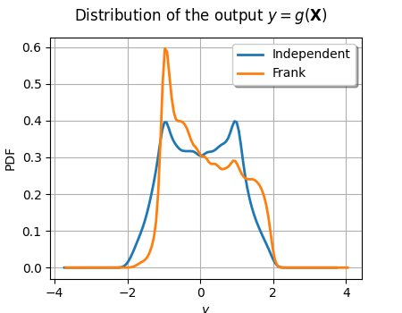
graph = ot.KernelSmoothing().build(outputSample_ind).drawPDF()
graph.setLegends(["Independent"])
graph.setTitle(r"Distribution of the output $y=g(\mathbf{X})$")
curve = ot.KernelSmoothing().build(outputSample_dep).drawPDF()
curve.setLegends(["Frank"])
graph.add(curve)
graph.setColors(ot.Drawable.BuildDefaultPalette(2))
view = otv.View(graph, figure_kw={"figsize": (4.5, 3.5)})
# view.save("kernel_output.pdf")

ThresholdEvent

threshold = 1.0  # Change this to 2.0 to turn it into a difficult problem
event = ot.ThresholdEvent(outputVect_ind, ot.Greater(), threshold)
event

class=ThresholdEventImplementation antecedent=class=CompositeRandomVector function=class=Function name=Unnamed implementation=class=FunctionImplementation name=Unnamed description=[$x_0$,$x_1$,$y$] evaluationImplementation=class=SymbolicEvaluation name=Unnamed inputVariablesNames=[x0,x1] outputVariablesNames=[y0] formulas=[sin(x0) * (1 + x1 ^ 2)] gradientImplementation=class=SymbolicGradient name=Unnamed evaluation=class=SymbolicEvaluation name=Unnamed inputVariablesNames=[x0,x1] outputVariablesNames=[y0] formulas=[sin(x0) * (1 + x1 ^ 2)] hessianImplementation=class=SymbolicHessian name=Unnamed evaluation=class=SymbolicEvaluation name=Unnamed inputVariablesNames=[x0,x1] outputVariablesNames=[y0] formulas=[sin(x0) * (1 + x1 ^ 2)] antecedent=class=UsualRandomVector distribution=class=JointDistribution name=JointDistribution dimension=2 copula=class=IndependentCopula name=IndependentCopula dimension=2 marginal[0]=class=Normal name=Normal dimension=1 mean=class=Point name=Unnamed dimension=1 values=[0] sigma=class=Point name=Unnamed dimension=1 values=[1] correlationMatrix=class=CorrelationMatrix dimension=1 implementation=class=MatrixImplementation name=Unnamed rows=1 columns=1 values=[1] marginal[1]=class=Uniform name=Uniform dimension=1 a=0 b=1 operator=class=Greater name=Unnamed threshold=1

maximumCoV = 0.05  # Coefficient of variation
maximumNumberOfBlocks = 100000
experiment = ot.MonteCarloExperiment()
algoMC = ot.ProbabilitySimulationAlgorithm(event, experiment)
algoMC.setMaximumOuterSampling(maximumNumberOfBlocks)
algoMC.setBlockSize(1)
algoMC.setMaximumCoefficientOfVariation(maximumCoV)

algoMC.run()

result = algoMC.getResult()
probability = result.getProbabilityEstimate()
print("Pf = ", probability)

Pf =  0.1497584541062803

otv.View.ShowAll()