Benchmark the Borehole test function

import openturns as ot
import otbenchmark as otb
import openturns.viewer as otv

problem = otb.BoreholeSensitivity()
print(problem)

name = Borehole
distribution = ComposedDistribution(Normal(mu = 0.1, sigma = 0.0161812), LogNormal(muLog = 7.71, sigmaLog = 1.0056, gamma = 0), Uniform(a = 63070, b = 115600), Uniform(a = 990, b = 1110), Uniform(a = 63.1, b = 116), Uniform(a = 700, b = 820), Uniform(a = 1120, b = 1680), Uniform(a = 9855, b = 12045), IndependentCopula(dimension = 8))
function = [rw,r,Tu,Hu,Tl,Hl,L,Kw]->[(2*pi_*Tu*(Hu-Hl))/(ln(r/rw)*(1+(2*L*Tu)/(ln(r/rw)*rw^2*Kw)+Tu/Tl))]
firstOrderIndices = [0.66,0,0,0.09,0,0.09,0.09,0.02]
totalOrderIndices = [0.69,0,0,0.11,0,0.11,0.1,0.02]

distribution = problem.getInputDistribution()
model = problem.getFunction()

Exact first and total order

exact_first_order = problem.getFirstOrderIndices()
exact_first_order

class=Point name=Unnamed dimension=8 values=[0.66,0,0,0.09,0,0.09,0.09,0.02]

exact_total_order = problem.getTotalOrderIndices()
exact_total_order

class=Point name=Unnamed dimension=8 values=[0.69,0,0,0.11,0,0.11,0.1,0.02]

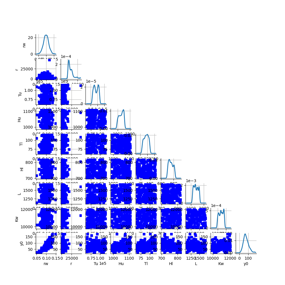
Plot the function

Create X/Y data

ot.RandomGenerator.SetSeed(0)
size = 200
inputDesign = ot.MonteCarloExperiment(distribution, size).generate()
outputDesign = model(inputDesign)

dimension = distribution.getDimension()
full_sample = ot.Sample(size, 1 + dimension)
full_sample[:, range(dimension)] = inputDesign
full_sample[:, dimension] = outputDesign
full_description = list(inputDesign.getDescription())
full_description.append(outputDesign.getDescription()[0])
full_sample.setDescription(full_description)

marginal_distribution = ot.ComposedDistribution(
    [
        ot.KernelSmoothing().build(full_sample.getMarginal(i))
        for i in range(1 + dimension)
    ]
)
clouds = ot.VisualTest.DrawPairsMarginals(full_sample, marginal_distribution)
_ = otv.View(clouds, figure_kw={"figsize": (10.0, 10.0)})

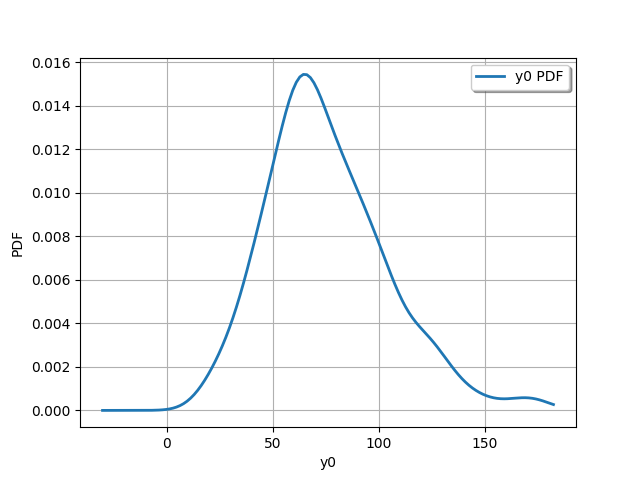
output_distribution = ot.KernelSmoothing().build(outputDesign)
_ = otv.View(output_distribution.drawPDF())

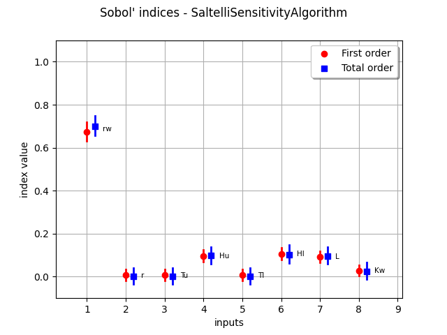
Perform sensitivity analysis

Create X/Y data

ot.RandomGenerator.SetSeed(0)
size = 10000
inputDesign = ot.SobolIndicesExperiment(distribution, size).generate()
outputDesign = model(inputDesign)

Compute first order indices using the Saltelli estimator

sensitivityAnalysis = ot.SaltelliSensitivityAlgorithm(inputDesign, outputDesign, size)
computed_first_order = sensitivityAnalysis.getFirstOrderIndices()
computed_total_order = sensitivityAnalysis.getTotalOrderIndices()

Compare with exact results

print("Sample size : ", size)
# First order
# Compute absolute error (the LRE cannot be computed,
# because S can be zero)
print("Computed first order = ", computed_first_order)
print("Exact first order = ", exact_first_order)
# Total order
print("Computed total order = ", computed_total_order)
print("Exact total order = ", exact_total_order)

Sample size :  10000
Computed first order =  [0.673759,0.00700637,0.00702324,0.0955299,0.00698057,0.106366,0.0916606,0.0283122]
Exact first order =  [0.66,0,0,0.09,0,0.09,0.09,0.02]
Computed total order =  [0.699598,-5.69378e-05,-3.20159e-08,0.0973057,9.79799e-05,0.103265,0.095226,0.0247122]
Exact total order =  [0.69,0,0,0.11,0,0.11,0.1,0.02]

_ = otv.View(sensitivityAnalysis.draw())

otv.View.ShowAll()