Benchmark the NLOscillator test function

import openturns as ot
import otbenchmark as otb
import openturns.viewer as otv

problem = otb.NLOscillatorSensitivity()
print(problem)

name = N.L. Oscillator
distribution = ComposedDistribution(ParametrizedDistribution(parameters = LogNormalMuSigma(mu = 21.5, sigma = 2.15, gamma = 0)), ParametrizedDistribution(parameters = LogNormalMuSigma(mu = 1.5, sigma = 0.15, gamma = 0)), ParametrizedDistribution(parameters = LogNormalMuSigma(mu = 0.01, sigma = 0.001, gamma = 0)), ParametrizedDistribution(parameters = LogNormalMuSigma(mu = 1, sigma = 0.2, gamma = 0)), ParametrizedDistribution(parameters = LogNormalMuSigma(mu = 0.01, sigma = 0.002, gamma = 0)), ParametrizedDistribution(parameters = LogNormalMuSigma(mu = 0.05, sigma = 0.02, gamma = 0)), ParametrizedDistribution(parameters = LogNormalMuSigma(mu = 0.02, sigma = 0.01, gamma = 0)), ParametrizedDistribution(parameters = LogNormalMuSigma(mu = 100, sigma = 10, gamma = 0)), IndependentCopula(dimension = 8))
function = class=PythonEvaluation name=OpenTURNSPythonFunction
firstOrderIndices = [0.4,0.03,0.09,0.18,0.12,0.05,0.05,0]
totalOrderIndices = [0.4,0.04,0.1,0.23,0.16,0.07,0.06,0.01]

distribution = problem.getInputDistribution()
model = problem.getFunction()

Exact first and total order

exact_first_order = problem.getFirstOrderIndices()
exact_first_order

class=Point name=Unnamed dimension=8 values=[0.4,0.03,0.09,0.18,0.12,0.05,0.05,0]

exact_total_order = problem.getTotalOrderIndices()
exact_total_order

class=Point name=Unnamed dimension=8 values=[0.4,0.04,0.1,0.23,0.16,0.07,0.06,0.01]

Plot the function

Create X/Y data

ot.RandomGenerator.SetSeed(0)
size = 200
inputDesign = ot.MonteCarloExperiment(distribution, size).generate()
outputDesign = model(inputDesign)

dimension = distribution.getDimension()
full_sample = ot.Sample(size, 1 + dimension)
full_sample[:, range(dimension)] = inputDesign
full_sample[:, dimension] = outputDesign
full_description = list(inputDesign.getDescription())
full_description.append(outputDesign.getDescription()[0])
full_sample.setDescription(full_description)

marginal_distribution = ot.ComposedDistribution(
    [
        ot.KernelSmoothing().build(full_sample.getMarginal(i))
        for i in range(1 + dimension)
    ]
)
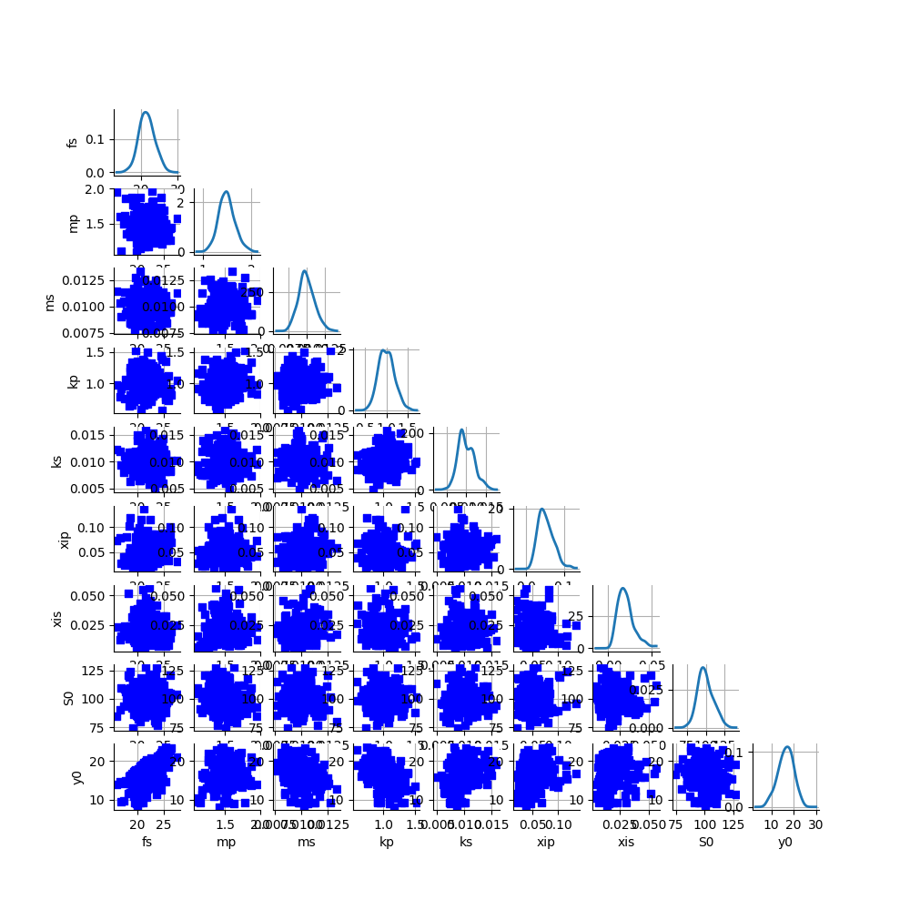
clouds = ot.VisualTest.DrawPairsMarginals(full_sample, marginal_distribution)
_ = otv.View(clouds, figure_kw={"figsize": (10.0, 10.0)})

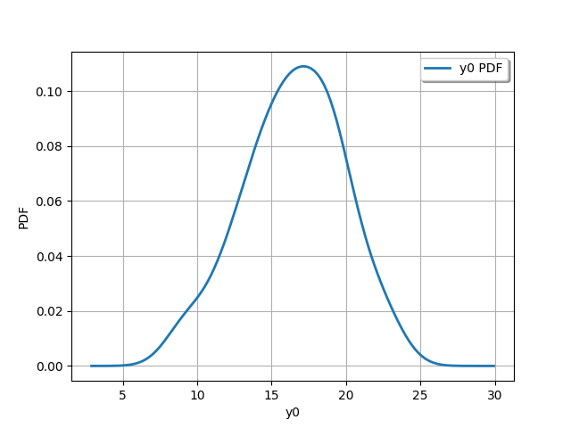
output_distribution = ot.KernelSmoothing().build(outputDesign)
_ = otv.View(output_distribution.drawPDF())

Perform sensitivity analysis

Create X/Y data

ot.RandomGenerator.SetSeed(0)
size = 10000
inputDesign = ot.SobolIndicesExperiment(distribution, size).generate()
outputDesign = model(inputDesign)

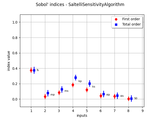
Compute first order indices using the Saltelli estimator

sensitivityAnalysis = ot.SaltelliSensitivityAlgorithm(inputDesign, outputDesign, size)
computed_first_order = sensitivityAnalysis.getFirstOrderIndices()
computed_total_order = sensitivityAnalysis.getTotalOrderIndices()

Compare with exact results

print("Sample size : ", size)
# First order
# Compute absolute error (the LRE cannot be computed,
# because S can be zero)
print("Computed first order = ", computed_first_order)
print("Exact first order = ", exact_first_order)
# Total order
print("Computed total order = ", computed_total_order)
print("Exact total order = ", exact_total_order)

Sample size :  10000
Computed first order =  [0.375093,0.0353727,0.0889049,0.17513,0.116545,0.0498364,0.0415787,0.00698915]
Exact first order =  [0.4,0.03,0.09,0.18,0.12,0.05,0.05,0]
Computed total order =  [0.374448,0.0757221,0.129792,0.272108,0.212897,0.065201,0.0561997,0.00716611]
Exact total order =  [0.4,0.04,0.1,0.23,0.16,0.07,0.06,0.01]

_ = otv.View(sensitivityAnalysis.draw())

otv.View.ShowAll()