Initialize FMUPointToFieldFunction

The interest of using FMUs in Python lies in the ease to change its input / parameter values. This notably enables to study the behavior of the FMU with uncertain inputs / parameters.

Initialization scripts can gather a large number of initial values. The use of initialization scripts (.mos files) is common in Dymola :

• to save the value of all the variables of a model after simulation,

• to restart simulation from a given point.

---

First, retrieve the path to the FMU deviation.fmu. Recall the epidemiological model is dynamic, i.e. its output evolves over time.

import otfmi.example.utility
import otfmi
import openturns as ot
from os.path import abspath
import openturns.viewer as viewer

path_fmu = otfmi.example.utility.get_path_fmu("epid")

The initialization script must be provided to FMUPointToFieldFunction constructor. We thus create it now (using Python for clarity).

Note

The initialization script can be automatically created in Dymola.

temporary_file = "initialization.mos"
with open(temporary_file, "w") as f:
    f.write("total_pop = 500;\n")
    f.write("healing_rate = 0.02;\n")

If no initial value is provided for an input / parameter, it is set to its default initial value (as set in the FMU).

We are interested in the model output during the 2 first seconds of simulation (which corresponds to a specific moment in the epidemic spreading). We must create the time grid on which the model output will be interpolated.

mesh = ot.RegularGrid(0.0, 0.1, 20)
meshSample = mesh.getVertices()
print(meshSample)

     [ t   ]
 0 : [ 0   ]
 1 : [ 0.1 ]
 2 : [ 0.2 ]
 3 : [ 0.3 ]
 4 : [ 0.4 ]
 5 : [ 0.5 ]
 6 : [ 0.6 ]
 7 : [ 0.7 ]
 8 : [ 0.8 ]
 9 : [ 0.9 ]
10 : [ 1   ]
11 : [ 1.1 ]
12 : [ 1.2 ]
13 : [ 1.3 ]
14 : [ 1.4 ]
15 : [ 1.5 ]
16 : [ 1.6 ]
17 : [ 1.7 ]
18 : [ 1.8 ]
19 : [ 1.9 ]

We can now build the FMUPointToFieldFunction. In the example below, we use the initialization script to fix the (non-default) values of total_pop and healing_rate in the FMU. We can thus observe the evolution of infected depending on the infection_rate.

function = otfmi.FMUPointToFieldFunction(
    mesh,
    path_fmu,
    inputs_fmu=["infection_rate"],
    outputs_fmu=["infected"],
    initialization_script=abspath("initialization.mos"),
    start_time=0.0,
    final_time=5.0,
)

total_pop and healing_rate values are defined in the initialization script, and remain constant over time. We can now set probability laws on the function input variable infection_rate to propagate its uncertainty through the model:

lawInfected = ot.Normal(0.01, 0.003)
inputSample = lawInfected.getSample(10)
outputProcessSample = function(inputSample)

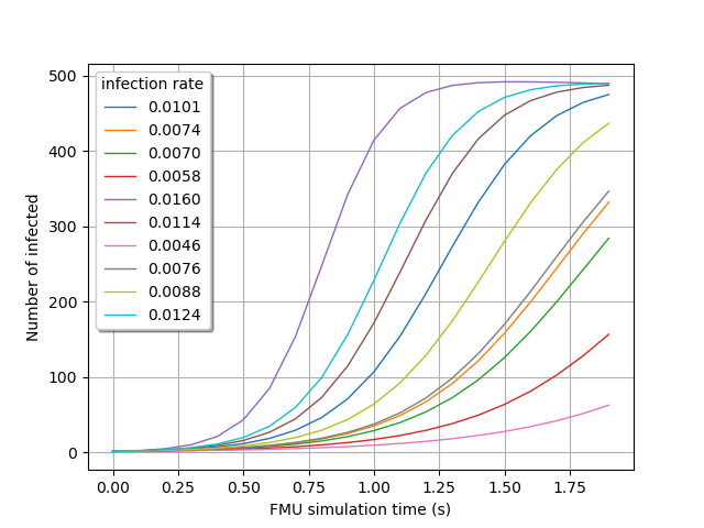
Visualize the time evolution of the infected over time, depending on the ìnfection_rate` value:

gridLayout = outputProcessSample.draw()
graph = gridLayout.getGraph(0, 0)
graph.setTitle("")
graph.setXTitle("FMU simulation time (s)")
graph.setYTitle("Number of infected")
graph.setLegends(["{:.4f}".format(line[0]) for line in inputSample])
view = viewer.View(graph, legend_kw={"title": "infection rate", "loc": "upper left"})
view.ShowAll()