View
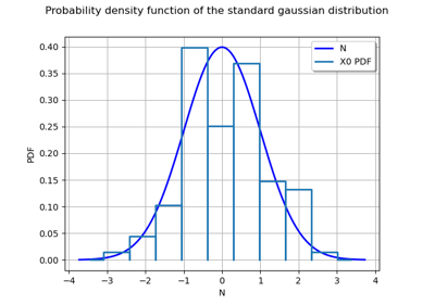
(Source code, png)
- class View(graph, pixelsize=None, figure=None, figure_kw=None, axes=[], plot_kw=None, axes_kw=None, bar_kw=None, pie_kw=None, polygon_kw=None, polygoncollection_kw=None, contour_kw=None, step_kw=None, clabel_kw=None, scatter_kw=None, text_kw=None, legend_kw=None, add_legend=True, square_axes=False, **kwargs)
Create the figure.
- Parameters:
- graph
Graph,DrawableorGridLayout An object to draw.
- pixelsize2-tuple of int
The requested size in pixels (width, height).
- figure
matplotlib.figure.Figure The figure to draw on.
- figure_kwdict, optional
Passed on to matplotlib.pyplot.figure kwargs
- axes
matplotlib.axes.Axes The axes to draw on.
- plot_kwdict, optional
Used when drawing Curve drawables Passed on as matplotlib.axes.Axes.plot kwargs
- axes_kwdict, optional
Passed on to matplotlib.figure.Figure.add_subplot kwargs
- bar_kwdict, optional
Used when drawing BarPlot drawables Passed on to matplotlib.pyplot.bar kwargs
- pie_kwdict, optional
Used when drawing Pie drawables Passed on to matplotlib.pyplot.pie kwargs
- polygon_kwdict, optional
Used when drawing Polygon drawables Passed on to matplotlib.patches.Polygon kwargs
- polygoncollection_kwdict, optional
Used when drawing PolygonArray drawables Passed on to matplotlib.collection.PolygonCollection kwargs
- contour_kwdict, optional
Used when drawing Contour drawables Passed on to matplotlib.pyplot.contour kwargs
- clabel_kwdict, optional
Used when drawing Contour drawables Passed on to matplotlib.pyplot.clabel kwargs
- scatter_kwdict, optional
Used when drawing Cloud drawables Passed on to matplotlib.pyplot.scatter kwargs
- step_kwdict, optional
Used when drawing Staircase drawables Passed on to matplotlib.pyplot.step kwargs
- text_kwdict, optional
Used when drawing Pairs, Text drawables Passed on to matplotlib.axes.Axes.text kwargs
- legend_kwdict, optional
Passed on to matplotlib.axes.Axes.legend kwargs
- add_legendbool, optional
Adds a legend if True. Default is True.
- square_axesbool, optional
Forces the axes to share the same scale if True. Default is False.
- graph
Methods
ShowAll(**kwargs)Display all graphs.
close()Close the figure.
getAxes()Get the matrix of Axes objects if the graph is a GridLayout, the list of Axes objects otherwise.
Get the list of QuadContourSet objects.
Accessor to the underlying figure object.
Get the matrix of View objects if the graph is GridLayout, None otherwise.
save(fname, **kwargs)Save the graph as file.
show(**kwargs)Display the graph.
Examples
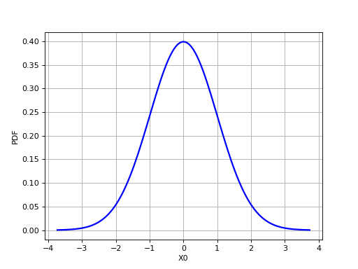
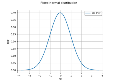
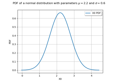
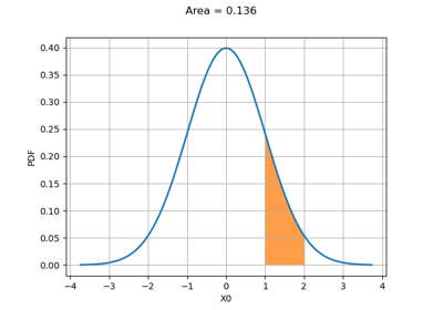
>>> import openturns as ot
>>> from openturns.viewer import View
>>> graph = ot.Normal().drawPDF()
>>> view = View(graph, plot_kw={'color':'blue'})
>>> view.save('graph.png', dpi=100)
>>> view.show()
- __init__(graph, pixelsize=None, figure=None, figure_kw=None, axes=[], plot_kw=None, axes_kw=None, bar_kw=None, pie_kw=None, polygon_kw=None, polygoncollection_kw=None, contour_kw=None, step_kw=None, clabel_kw=None, scatter_kw=None, text_kw=None, legend_kw=None, add_legend=True, square_axes=False, **kwargs)
- static ShowAll(**kwargs)
Display all graphs.
Examples
>>> import openturns as ot
>>> import openturns.viewer as otv
>>> n = ot.Normal()
>>> graph = n.drawPDF()
>>> view = otv.View(graph)
>>> u = ot.Uniform()
>>> graph = u.drawPDF()
>>> view = otv.View(graph)
>>> otv.View.ShowAll()
- close()
Close the figure.
Examples
>>> import openturns as ot
>>> import openturns.viewer as otv
>>> n = ot.Normal()
>>> graph = n.drawPDF()
>>> view = otv.View(graph)
>>> view.close()
- getAxes()
Get the matrix of Axes objects if the graph is a GridLayout, the list of Axes objects otherwise.
See matplotlib.axes.Axes for further information.
Examples
>>> import openturns as ot
>>> import openturns.viewer as otv
>>> n = ot.Normal()
>>> graph = n.drawPDF()
>>> view = otv.View(graph)
>>> axes = view.getAxes()
>>> _ = axes[0].set_ylim(-0.1, 1.0);
- getContourSets()
Get the list of QuadContourSet objects.
See matplotlib.contour.QuadContourSet for further information.
Examples
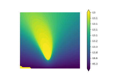
>>> import openturns as ot
>>> import openturns.viewer as otv
>>> f = ot.SymbolicFunction(['x', 'y'], ['exp(-sin(cos(y)^2*x^2+sin(x)^2*y^2))'])
>>> view = otv.View(f.draw([0.,0.],[10.,10.],[50]*2))
>>> contoursets = view.getContourSets()
>>> colorbar = view.getFigure().colorbar(contoursets[0]);
- getFigure()
Accessor to the underlying figure object.
See matplotlib.figure.Figure for further information.
Examples
>>> import openturns as ot
>>> from openturns.viewer import View
>>> graph = ot.Normal().drawPDF()
>>> view = View(graph)
>>> fig = view.getFigure()
>>> _ = fig.suptitle("The suptitle");
- getSubviews()
Get the matrix of View objects if the graph is GridLayout, None otherwise.
Examples
>>> import openturns as ot
>>> import openturns.viewer as otv
>>> f = ot.SymbolicFunction(['x', 'y'], ['exp(-sin(cos(y)^2*x^2+sin(x)^2*y^2))'])
>>> grid = ot.GridLayout(1, 2)
>>> grid.setGraphCollection(ot.graph._GraphCollection([f.draw(0, 0, [0., 0.], 0., 10., 50), f.draw([0., 0.], [10., 10.], [50]*2)]))
>>> view = otv.View(grid)
>>> colorbar = view.getFigure().colorbar(view.getSubviews()[0][1].getContourSets()[0])
- save(fname, **kwargs)
Save the graph as file.
- Parameters:
- fnamebool, optional
A string containing a path to a filename from which file format is deduced.
- kwargsdict
See matplotlib.figure.Figure.savefig documentation for valid keyword arguments.
Examples
>>> import openturns as ot
>>> from openturns.viewer import View
>>> graph = ot.Normal().drawPDF()
>>> view = View(graph)
>>> view.save('graph.png', dpi=100)
- show(**kwargs)
Display the graph.
See matplotlib.figure.Figure.show
Examples
>>> import openturns as ot
>>> import openturns.viewer as otv
>>> n = ot.Normal()
>>> graph = n.drawPDF()
>>> view = otv.View(graph)
>>> view.show()
Examples using the class
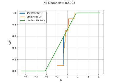
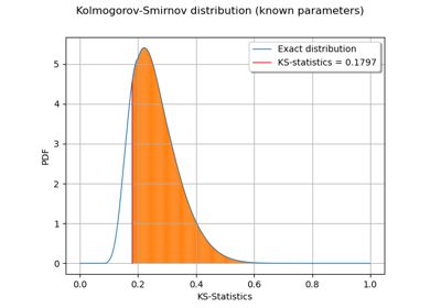
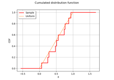
Kolmogorov-Smirnov : get the statistics distribution
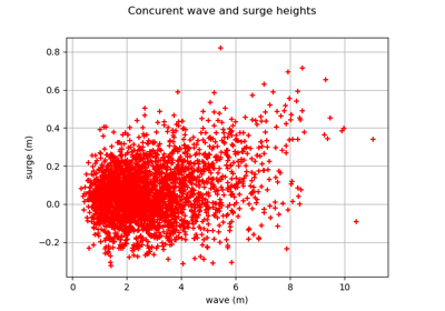
Estimate tail dependence coefficients on the wave-surge data
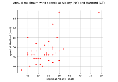
Estimate tail dependence coefficients on the wind data
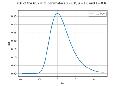
Create the distribution of the maximum of independent distributions
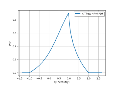
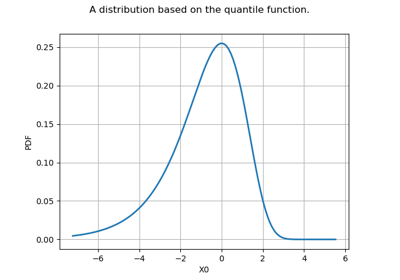
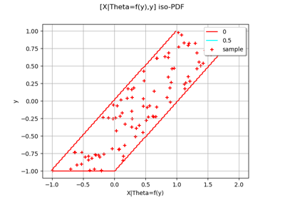
Create your own distribution given its quantile function


Create a process from random vectors and processes
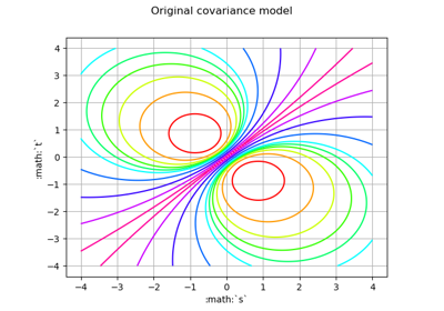
Sample trajectories from a Gaussian Process with correlated outputs
Create a polynomial chaos metamodel by integration on the cantilever beam
Create a polynomial chaos metamodel from a data set
Create a polynomial chaos for the Ishigami function: a quick start guide to polynomial chaos
Conditional expectation of a polynomial chaos expansion
Gaussian Process Regression : cantilever beam model
Example of multi output Kriging on the fire satellite model
Kriging: choose a polynomial trend on the beam model
Evaluate the mean of a random vector by simulations
Estimate a probability with Monte-Carlo on axial stressed beam: a quick start guide to reliability
Use the FORM algorithm in case of several design points
Non parametric Adaptive Importance Sampling (NAIS)

Axial stressed beam : comparing different methods to estimate a probability
An illustrated example of a FORM probability estimate
Estimate Sobol indices on a field to point function
Sobol’ sensitivity indices using rank-based algorithm
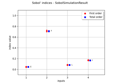
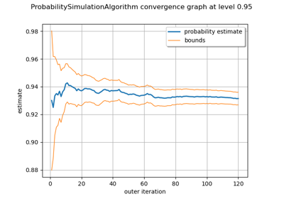
Estimate Sobol’ indices for the beam by simulation algorithm
Estimate Sobol’ indices for a function with multivariate output
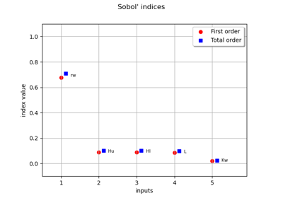
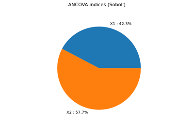
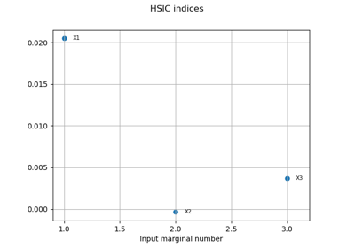
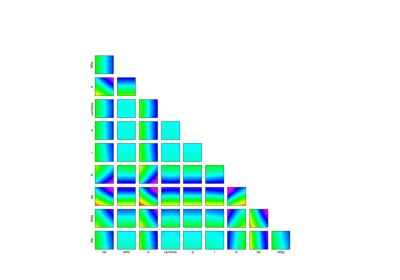
Example of sensitivity analyses on the wing weight model
Create mixed deterministic and probabilistic designs of experiments
Create a design of experiments with discrete and continuous variables
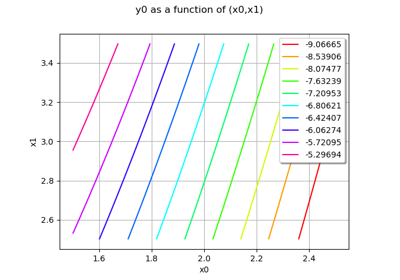
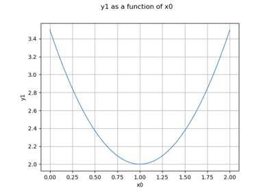
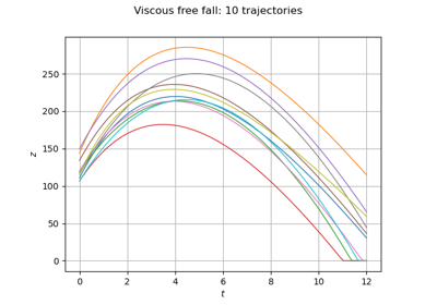
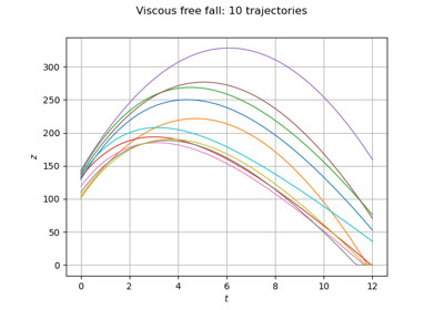
Define a function with a field output: the viscous free fall example

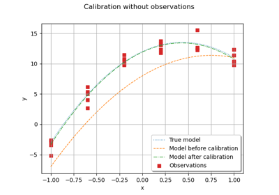
Calibrate a parametric model: a quick-start guide to calibration
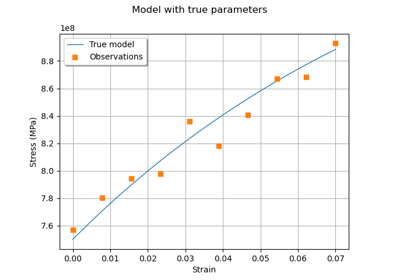
Generate observations of the Chaboche mechanical model
Linear Regression with interval-censored observations
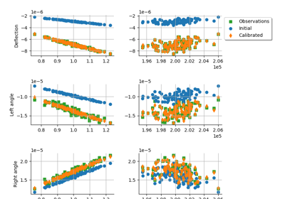
Bayesian calibration of hierarchical fission gas release models

Estimate a multivariate integral with IteratedQuadrature
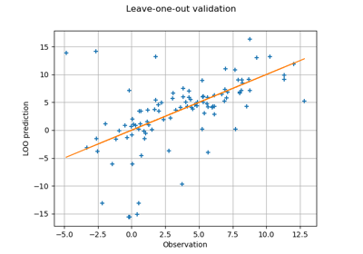
Compute leave-one-out error of a polynomial chaos expansion
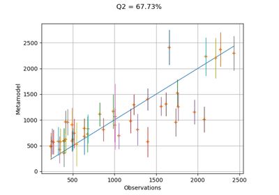
Compute confidence intervals of a regression model from data
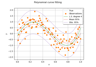
Compute confidence intervals of a univariate noisy function
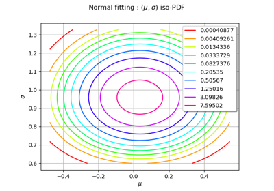
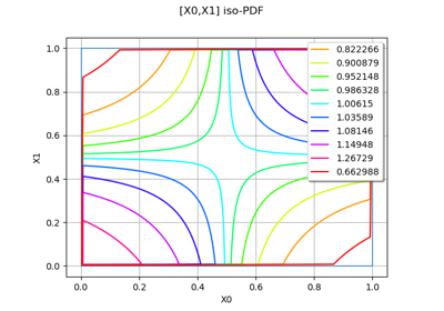
Plot the log-likelihood contours of a distribution