Initialize FMUPointToFieldFunction

The interest of using FMUs in Python lies in the ease to change its input / parameter values. This notably enables to study the behavior of the FMU with uncertain inputs / parameters.

Initialization scripts can gather a large number of initial values. The use of initialization scripts (.mos files) is common in Dymola :

• to save the value of all the variables of a model after simulation,

• to restart simulation from a given point.

First, retrieve the path to the FMU deviation.fmu.

import otfmi.example.utility
import otfmi
import openturns as ot
from os.path import abspath
import openturns.viewer as viewer

path_fmu = otfmi.example.utility.get_path_fmu("epid")

The initialization script must be provided to FMUPointToFieldFunction constructor. We thus create it now (using Python for clarity).

Note

The initialization script can be automatically created in Dymola.

temporary_file = "initialization.mos"
with open(temporary_file, "w") as f:
    f.write("total_pop = 500;\n")
    f.write("healing_rate = 0.5;\n")

If no initial value is provided for an input / parameter, it is set to its default initial value (as set in the FMU).

We are interested in the model output during the 2 first seconds of simulation (which corresponds to a specific moment in the epidemic spreading). We must create the time grid on which the model output will be interpolated.

mesh = ot.RegularGrid(0.0, 0.1, 20)
meshSample = mesh.getVertices()
print(meshSample)

     [ t   ]
 0 : [ 0   ]
 1 : [ 0.1 ]
 2 : [ 0.2 ]
 3 : [ 0.3 ]
 4 : [ 0.4 ]
 5 : [ 0.5 ]
 6 : [ 0.6 ]
 7 : [ 0.7 ]
 8 : [ 0.8 ]
 9 : [ 0.9 ]
10 : [ 1   ]
11 : [ 1.1 ]
12 : [ 1.2 ]
13 : [ 1.3 ]
14 : [ 1.4 ]
15 : [ 1.5 ]
16 : [ 1.6 ]
17 : [ 1.7 ]
18 : [ 1.8 ]
19 : [ 1.9 ]

We can now build the FMUPointToFieldFunction. In the example below, we use the initialization script to fix the (non-default) values of total_pop and healing_rate in the FMU. We can thus observe the evolution of infected depending on the infection_rate.

function = otfmi.FMUPointToFieldFunction(
    path_fmu,
    mesh,
    inputs_fmu=["infection_rate"],
    outputs_fmu=["infected"],
    initialization_script=abspath("initialization.mos"),
    start_time=0.0,
    final_time=5.0,
)

total_pop and healing_rate values are defined in the initialization script, and remain constant over time. We can now set probability laws on the function input variable infection_rate to propagate its uncertainty through the model:

law_infection_rate = ot.Normal(2.0, 0.25)
inputSample = law_infection_rate.getSample(10)
outputProcessSample = function(inputSample)

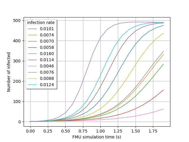
Visualize the time evolution of the infected over time, depending on the ìnfection_rate` value:

gridLayout = outputProcessSample.draw()
graph = gridLayout.getGraph(0, 0)
graph.setTitle("")
graph.setXTitle("FMU simulation time (s)")
graph.setYTitle("Number of infected")
graph.setLegends([f"{line[0]:.4f}" for line in inputSample])
view = viewer.View(graph, legend_kw={"title": "infection rate", "loc": "upper left"})
view.ShowAll()