ParetoFactory¶

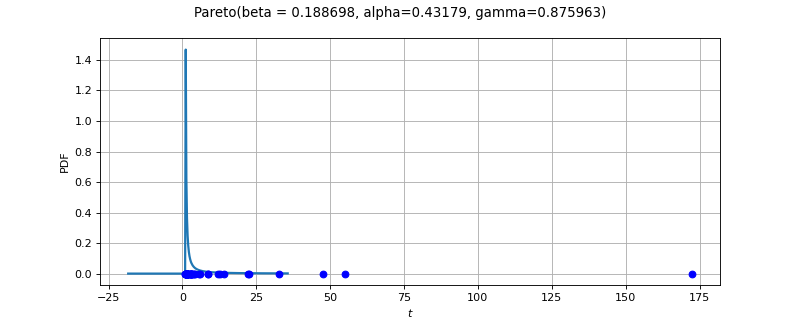
(Source code, png)

class ParetoFactory(*args)¶

Pareto factory.

Methods

`build`(*args)	Build the distribution.
`buildAsPareto`(*args)	Estimate the distribution as native distribution.
`buildEstimator`(*args)	Build the distribution and the parameter distribution.
`buildMethodOfLeastSquares`(*args)	Method of least-squares.
`buildMethodOfLikelihoodMaximization`(sample)	Method of likelihood maximization.
`buildMethodOfMoments`(sample)	Method of moments estimator.
`getBootstrapSize`()	Accessor to the bootstrap size.
`getClassName`()	Accessor to the object's name.
`getKnownParameterIndices`()	Accessor to the known parameters indices.
`getKnownParameterValues`()	Accessor to the known parameters values.
`getName`()	Accessor to the object's name.
`hasName`()	Test if the object is named.
`setBootstrapSize`(bootstrapSize)	Accessor to the bootstrap size.
`setKnownParameter`(values, positions)	Accessor to the known parameters.
`setName`(name)	Accessor to the object's name.

See also

DistributionFactory, Normal

Notes

Several estimators to build a Pareto distribution from a scalar sample are proposed. The default strategy is to use the least squares estimator.

Moments based estimator:

Lets denote:

$\displaystyle \overline{x}_n = \frac{1}{n} \sum_{i=1}^n x_i$ the empirical mean of the sample,
$\displaystyle s_n^2 = \frac{1}{n-1} \sum_{i=1}^n (x_i - \overline{x}_n)^2$ its empirical variance,
$\displaystyle skew_n$ the empirical skewness of the sample

The estimator $(\hat{\beta}_n, \hat{\alpha}_n, \hat{\gamma}_n)$ of $(\beta, \alpha, \gamma)$ is defined as follows :

The parameter $\hat{\alpha}_n$ is solution of the equation:

$\begin{eqnarray*} skew_n & = & \dfrac{ 2(1+\hat{\alpha}_n) }{ \hat{\alpha}_n-3 } \sqrt{ \dfrac{ \hat{\alpha}_n-2 }{ \hat{\alpha}_n } } \end{eqnarray*}$

There exists a symbolic solution. If $\hat{\alpha}_n >3$ , then we get $(\hat{\beta}_n, \hat{\gamma}_n)$ as follows:

$\begin{eqnarray*} \hat{\beta}_n & = & (\hat{\alpha}_n-1) \sqrt{\dfrac{\hat{\alpha}_n-2}{\hat{\alpha}_n}}s_n \\ \hat{\gamma}_n & = & \overline{x}_n - \dfrac{\hat{\alpha}_n}{\hat{\alpha}_n+1} \hat{\beta}_n \end{eqnarray*}$

Maximum likelihood based estimator:

The likelihood of the sample is defined by:

$\ell(\alpha, \beta, \gamma| x_1, \dots, x_n) = n\log \alpha + n\alpha \log \beta - (\alpha+1) \sum_{i=1}^n \log(x_i-\gamma)$

The maximum likelihood based estimator $(\hat{\beta}_n, \hat{\alpha}_n, \hat{\gamma}_n)$ of $(\beta, \alpha, \gamma)$ maximizes the likelihood:

$(\hat{\beta}_n, \hat{\alpha}_n, \hat{\gamma}_n) = \argmax_{\alpha, \beta, \gamma} \ell(\alpha, \beta, \gamma| x_1, \dots, x_n)$

The following strategy is to be implemented soon: For a given $\gamma$ , the likelihood of the sample is defined by:

$\ell(\alpha(\gamma), \beta(\gamma)| x_1, \dots, x_n, \gamma) = n\log \alpha(\gamma) + n\alpha(\gamma) \log \beta(\gamma) - (\alpha(\gamma)+1) \sum_{i=1}^n \log(x_i-\gamma)$

We get $(\hat{\beta}_n( \gamma), \hat{\alpha}_n( \gamma))$ which maximizes $\ell(\alpha, \beta| x_1, \dots, x_n, \gamma)$ :

$(\hat{\beta}_n( \gamma), \hat{\alpha}_n( \gamma)) = \argmax_{\alpha, \beta} \ell(\alpha(\gamma), \beta(\gamma)| x_1, \dots, x_n, \gamma) \text{ under the constraint } \gamma + \hat{\beta}_n(\gamma) \leq x_{(1,n)}$

We get:

$\begin{eqnarray*} \hat{\beta}_n( \gamma) & = & x_{(1,n)} - \gamma \\ \hat{\alpha}_n( \gamma) & = & \dfrac{n}{\sum_{i=1}^n \log\left( \dfrac{x_i - \gamma}{\hat{\beta}_n( \gamma)}\right)} \end{eqnarray*}$

Then the parameter $\gamma$ is obtained by maximizing the likelihood $\ell(\hat{\beta}_n( \gamma), \hat{\alpha}_n( \gamma), \gamma)$ :

$\hat{\gamma}_n = \argmax_{\gamma} \ell(\hat{\beta}_n( \gamma), \hat{\alpha}_n( \gamma), \gamma)$

The initial point of the optimisation problem is $\gamma_0 = x_{(1,n)} - |x_{(1,n)}|/(2+n)$ .

Least squares estimator:

The parameter $\gamma$ is numerically optimized by non-linear least-squares:

$\min{\gamma} \norm{\hat{S}_n(x_i) - (a_1 \log(x_i - \gamma) + a_0)}_2^2$

where $a_0, a_1$ are computed from linear least-squares at each optimization evaluation.

When $\gamma$ is known and the $x_i$ follow a Pareto distribution then we use linear least-squares to solve the relation:

(1)¶ $\hat{S}_n(x_i) = a_1 \log(x_i - \gamma) + a_0$

And the remaining parameters are estimated with:

$\hat{\beta} &= \exp{\frac{-a_0}{a_1}}\\ \hat{\alpha} &= -a_1$

__init__(*args)¶

build(*args)¶

Build the distribution.

Available usages:

build()

build(sample)

build(param)

Parameters:

sample2-d sequence of float: Data.
paramsequence of float: The parameters of the distribution.

Returns:

distDistribution

The estimated distribution.

In the first usage, the default native distribution is built.

buildAsPareto(*args)¶

Estimate the distribution as native distribution.

Available usages:

buildAsPareto()

buildAsPareto(sample)

buildAsPareto(param)

Parameters:

sample2-d sequence of float: Data.
paramsequence of float,: The parameters of the Pareto.

Returns:

distPareto

The estimated distribution as a Pareto.

In the first usage, the default Pareto distribution is built.

buildEstimator(*args)¶

Build the distribution and the parameter distribution.

Parameters:

sample2-d sequence of float: Data.
parametersDistributionParameters: Optional, the parametrization.

Returns:

resDistDistributionFactoryResult: The results.

Notes

According to the way the native parameters of the distribution are estimated, the parameters distribution differs:

Moments method: the asymptotic parameters distribution is normal and estimated by Bootstrap on the initial data;

Maximum likelihood method with a regular model: the asymptotic parameters distribution is normal and its covariance matrix is the inverse Fisher information matrix;

Other methods: the asymptotic parameters distribution is estimated by Bootstrap on the initial data and kernel fitting (see KernelSmoothing).

If another set of parameters is specified, the native parameters distribution is first estimated and the new distribution is determined from it:

if the native parameters distribution is normal and the transformation regular at the estimated parameters values: the asymptotic parameters distribution is normal and its covariance matrix determined from the inverse Fisher information matrix of the native parameters and the transformation;

in the other cases, the asymptotic parameters distribution is estimated by Bootstrap on the initial data and kernel fitting.

buildMethodOfLeastSquares(*args)¶

Method of least-squares.

Parameters:

sample2-d sequence of float: Data.
gammafloat, optional: Gamma parameter.

Returns:

distributionPareto: The estimated distribution.

Notes

Refer to LeastSquaresDistributionFactory.

buildMethodOfLikelihoodMaximization(sample)¶

Method of likelihood maximization.

Refer to MaximumLikelihoodFactory.

Parameters:

sample2-d sequence of float: Data.

Returns:

distributionPareto: The estimated distribution

buildMethodOfMoments(sample)¶

Method of moments estimator.

Parameters:

sample2-d sequence of float: Data.

Returns:

distributionPareto: The estimated distribution

getBootstrapSize()¶

Accessor to the bootstrap size.

Returns:

sizeint: Size of the bootstrap.

getClassName()¶

Accessor to the object’s name.

Returns:

class_namestr: The object class name (object.__class__.__name__).

getKnownParameterIndices()¶

Accessor to the known parameters indices.

Returns:

indicesIndices: Indices of the known parameters.

getKnownParameterValues()¶

Accessor to the known parameters values.

Returns:

valuesPoint: Values of known parameters.

getName()¶

Accessor to the object’s name.

Returns:

namestr: The name of the object.

hasName()¶

Test if the object is named.

Returns:

hasNamebool: True if the name is not empty.

setBootstrapSize(bootstrapSize)¶

Accessor to the bootstrap size.

Parameters:

sizeint: The size of the bootstrap.

setKnownParameter(values, positions)¶

Accessor to the known parameters.

Parameters:

valuessequence of float: Values of known parameters.
positionssequence of int: Indices of known parameters.

Examples

When a subset of the parameter vector is known, the other parameters only have to be estimated from data.

In the following example, we consider a sample and want to fit a Beta distribution. We assume that the $a$ and $b$ parameters are known beforehand. In this case, we set the third parameter (at index 2) to -1 and the fourth parameter (at index 3) to 1.

>>> import openturns as ot
>>> ot.RandomGenerator.SetSeed(0)
>>> distribution = ot.Beta(2.3, 2.2, -1.0, 1.0)
>>> sample = distribution.getSample(10)
>>> factory = ot.BetaFactory()
>>> # set (a,b) out of (r, t, a, b)
>>> factory.setKnownParameter([-1.0, 1.0], [2, 3])
>>> inf_distribution = factory.build(sample)