Distribution of estimators in linear regression

Introduction

In this example, we are interested in the distribution of the estimator of the variance of the observation error in linear regression. We are also interested in the estimator of the standard deviation of the observation error. We show how to use the PythonRandomVector class in order to perform a study of the sample distribution of these estimators.

In the general linear regression model, the observation error has the normal distribution where is the standard deviation. We are interested in the estimators of the variance and the standard deviation :

• the variance of the residuals, , is estimated from getResidualsVariance();

• the standard deviation is estimated from getResidualsStandardError().

The asymptotic distribution of these estimators is known (see [vaart2000]) but we want to perform an empirical study, based on simulation. In order to see the distribution of the estimator, we simulate an observation of the estimator, and repeat that experiment times, where is a large integer. Then we approximate the distribution using KernelSmoothing.

import openturns as ot
import openturns.viewer as otv
import pylab as pl

The simulation engine

The simulation is based on the PythonRandomVector class, which simulates independent observations of a random vector. The getRealization() method implements the simulation of the observation of the estimator.

class SampleEstimatorLinearRegression(ot.PythonRandomVector):
    def __init__(
        self, sample_size, true_standard_deviation, coefficients, estimator="variance"
    ):
        """
        Create a RandomVector for an estimator from a linear regression model.

        Parameters
        ----------
        sample_size : int
            The sample size n.
        true_standard_deviation : float
            The standard deviation of the Gaussian observation error.
        coefficients: sequence of p floats
            The coefficients of the linear model.
        estimator: str
            The estimator.
            Available estimators are "variance" or "standard-deviation".
        """
        super(SampleEstimatorLinearRegression, self).__init__(1)
        self.sample_size = sample_size
        self.numberOfParameters = coefficients.getDimension()
        input_dimension = self.numberOfParameters - 1  # Because of the intercept
        centerCoefficient = [0.0] * input_dimension
        constantCoefficient = [coefficients[0]]
        linearCoefficient = ot.Matrix([coefficients[1:]])
        self.linearModel = ot.LinearFunction(
            centerCoefficient, constantCoefficient, linearCoefficient
        )
        self.distribution = ot.Normal(input_dimension)
        self.distribution.setDescription(["x%d" % (i) for i in range(input_dimension)])
        self.errorDistribution = ot.Normal(0.0, true_standard_deviation)
        self.estimator = estimator
        # In classical linear regression, the input is deterministic.
        # Here, we set it once and for all.
        self.input_sample = self.distribution.getSample(self.sample_size)
        self.output_sample = self.linearModel(self.input_sample)

    def getRealization(self):
        errorSample = self.errorDistribution.getSample(self.sample_size)
        noisy_output_sample = self.output_sample + errorSample
        algo = ot.LinearModelAlgorithm(self.input_sample, noisy_output_sample)
        lmResult = algo.getResult()
        if self.estimator == "variance":
            output = lmResult.getResidualsVariance()
        elif self.estimator == "standard-deviation":
            lmAnalysis = ot.LinearModelAnalysis(lmResult)
            output = lmAnalysis.getResidualsStandardError()
        else:
            raise ValueError("Unknown estimator %s" % (self.estimator))
        return [output]


def plot_sample_by_kernel_smoothing(
    sample_size, true_standard_deviation, coefficients, estimator, repetitions_size
):
    """
    Plot the estimated distribution of the biased sample variance from a sample

    The method uses Kernel Smoothing with default kernel.

    Parameters
    ----------
    repetitions_size : int
        The number of repetitions of the experiments.
        This is the (children) size of the sample of the biased
        sample variance

    Returns
    -------
    graph : ot.Graph
        The plot of the PDF of the estimated distribution.

    """
    myRV = ot.RandomVector(
        SampleEstimatorLinearRegression(
            sample_size, true_standard_deviation, coefficients, estimator
        )
    )
    sample_estimator = myRV.getSample(repetitions_size)
    if estimator == "variance":
        sample_estimator.setDescription([r"$\hat{\sigma}^2$"])
    elif estimator == "standard-deviation":
        sample_estimator.setDescription([r"$\hat{\sigma}$"])
    else:
        raise ValueError("Unknown estimator %s" % (estimator))
    mean_sample_estimator = sample_estimator.computeMean()

    graph = ot.KernelSmoothing().build(sample_estimator).drawPDF()
    graph.setLegends(["Sample"])
    bb = graph.getBoundingBox()
    ylb = bb.getLowerBound()[1]
    yub = bb.getUpperBound()[1]
    curve = ot.Curve([true_standard_deviation**2] * 2, [ylb, yub])
    curve.setLegend("Exact")
    curve.setLineWidth(2.0)
    graph.add(curve)
    graph.setTitle(
        "Size = %d, True S.D. = %.4f, Mean = %.4f, Rep. = %d"
        % (
            sample_size,
            true_standard_deviation,
            mean_sample_estimator[0],
            repetitions_size,
        )
    )
    return graph

Distribution of the variance estimator

We first consider the estimation of the variance . In the next cell, we consider a sample size equal to with parameters. We use repetitions.

repetitions_size = 1000
true_standard_deviation = 0.1
sample_size = 6
coefficients = ot.Point([3.0, 2.0, -1.0])
estimator = "variance"
view = otv.View(
    plot_sample_by_kernel_smoothing(
        sample_size, true_standard_deviation, coefficients, estimator, repetitions_size
    ),
    figure_kw={"figsize": (6.0, 3.5)},
)
pl.subplots_adjust(bottom=0.25)

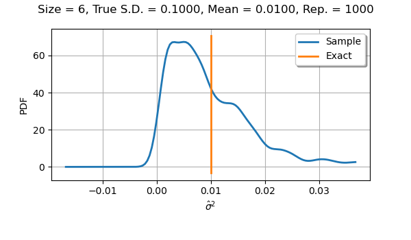
If we use a sample size equal to with parameters, the distribution is not symmetric. The mean of the observations of the sample variances remains close to the true value .

Then we increase the sample size .

repetitions_size = 1000
true_standard_deviation = 0.1
sample_size = 100
coefficients = ot.Point([3.0, 2.0, -1.0])
view = otv.View(
    plot_sample_by_kernel_smoothing(
        sample_size, true_standard_deviation, coefficients, estimator, repetitions_size
    ),
    figure_kw={"figsize": (6.0, 3.5)},
)
pl.subplots_adjust(bottom=0.25)

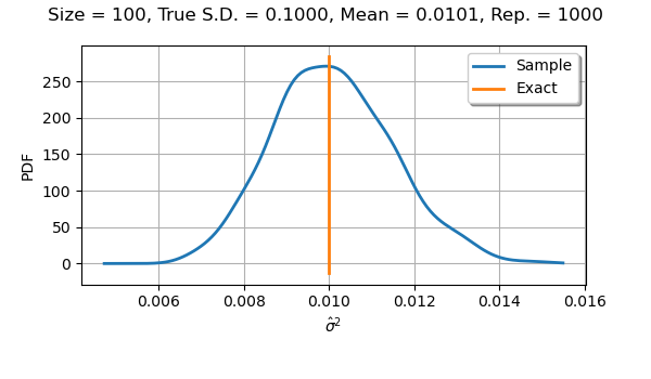
If we use a sample size equal to with parameters, the distribution is almost symmetric and almost normal.

Distribution of the standard deviation estimator

We now consider the estimation of the standard deviation .

repetitions_size = 1000
true_standard_deviation = 0.1
sample_size = 6
coefficients = ot.Point([3.0, 2.0, -1.0])
estimator = "standard-deviation"
view = otv.View(
    plot_sample_by_kernel_smoothing(
        sample_size, true_standard_deviation, coefficients, estimator, repetitions_size
    ),
    figure_kw={"figsize": (6.0, 3.5)},
)
pl.subplots_adjust(bottom=0.25)

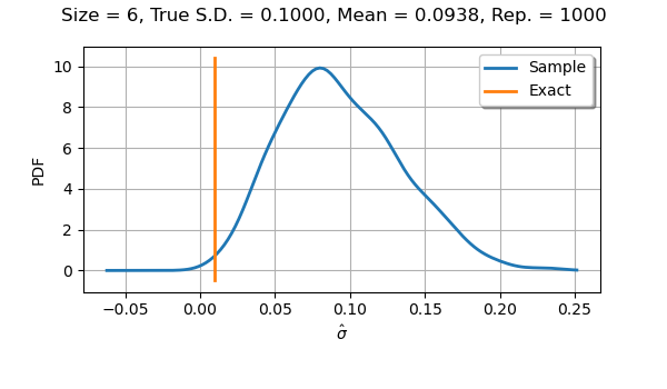
If we use a sample size equal to with parameters, we see that the distribution is almost symmetric. We notice a slight bias, since the mean of the observations of the standard deviation is not as close to the true value 0.1 as we could expect.

repetitions_size = 1000
true_standard_deviation = 0.1
sample_size = 100
coefficients = ot.Point([3.0, 2.0, -1.0])
estimator = "standard-deviation"
view = otv.View(
    plot_sample_by_kernel_smoothing(
        sample_size, true_standard_deviation, coefficients, estimator, repetitions_size
    ),
    figure_kw={"figsize": (6.0, 3.5)},
)
pl.subplots_adjust(bottom=0.25)

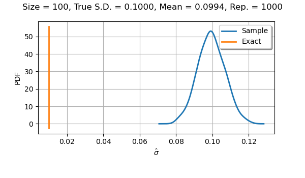
If we use a sample size equal to with parameters, we see that the distribution is almost normal. We notice that the bias disappeared.