LinearModelAnalysis
- class LinearModelAnalysis(*args)
Analyse a linear model.
- Parameters:
- linearModelResult
LinearModelResult A linear model result.
- linearModelResult
Methods
Accessor to plot of Cook's distances versus row labels.
Accessor to plot of Cook's distances versus leverage/(1-leverage).
Accessor to plot of model versus fitted values.
Accessor to plot a Normal quantiles-quantiles plot of standardized residuals.
Accessor to plot of residuals versus fitted values.
Accessor to plot of residuals versus leverages that adds bands corresponding to Cook's distances of 0.5 and 1.
Accessor to a Scale-Location plot of sqrt(abs(residuals)) versus fitted values.
Accessor to the object's name.
getCoefficientsConfidenceInterval([level])Accessor to the confidence interval of level
 for the coefficients of the linear expansion
Accessor to the coefficients of the p values.
Accessor to the coefficients of linear expansion over their standard error.
Accessor to the Fisher p value.
Accessor to the Fisher statistics.
Accessor to the linear model result.
getName()Accessor to the object's name.
Performs Cramer-Von Mises test.
Performs Anderson-Darling test.
Performs Chi-Square test.
Performs Kolmogorov test.
Accessor to the standard error of the residuals.
hasName()Test if the object is named.
setName(name)Accessor to the object's name.
See also
Notes
This class relies on a linear model result structure and analyses the results.
By default, on graphs, labels of the 3 most significant points are displayed. This number can be changed by modifying the ResourceMap key (
LinearModelAnalysis-IdentifiersNumber).The class has a pretty-print method which is triggered by the print() function. This prints the following results, where we focus on the properties of a satisfactory regression model.
Each row of the table of coefficients tests if one single coefficient is zero. For a single coefficient, if the p-value of the T-test is close to zero, we can reject the hypothesis that this coefficient is zero.
The R2 score measures how the predicted output values are close to the observed values. If the R2 is close to 1 (e.g. larger than 0.95), then the predictions are accurate on average. Furthermore, the adjusted R2 value takes into account the data set size and the number of hyperparameters.
The F-test tests if all the coefficients are simultaneously zero. If the p-value is close to zero, then we can reject this hypothesis: there is at least one nonzero coefficient.
The normality test checks that the residuals have a normal distribution. The normality assumption can be accepted (or, more precisely, cannot be rejected) if the p-value is larger than a threshold (e.g. 0.05).
The essentials of regression theory are presented in Regression analysis. The goodness of fit tests for normality are presented in Graphical goodness-of-fit tests, Chi-squared test, The Kolmogorov-Smirnov goodness of fit test for continuous data, Cramer-Von Mises test and Anderson-Darling test.
Examples
>>> import openturns as ot
>>> ot.RandomGenerator.SetSeed(0)
>>> distribution = ot.Normal()
>>> Xsample = distribution.getSample(30)
>>> func = ot.SymbolicFunction(['x'], ['2 * x + 1'])
>>> Ysample = func(Xsample) + ot.Normal().getSample(30)
>>> algo = ot.LinearModelAlgorithm(Ysample, Xsample)
>>> result = algo.getResult()
>>> analysis = ot.LinearModelAnalysis(result)
>>> # print(analysis)  # Pretty-print
- __init__(*args)
- drawCookVsLeverages()
Accessor to plot of Cook’s distances versus leverage/(1-leverage).
- Returns:
- graph
Graph
- graph
- drawQQplot()
Accessor to plot a Normal quantiles-quantiles plot of standardized residuals.
- Returns:
- graph
Graph
- graph
- drawResidualsVsLeverages()
Accessor to plot of residuals versus leverages that adds bands corresponding to Cook’s distances of 0.5 and 1.
- Returns:
- graph
Graph
- graph
- drawScaleLocation()
Accessor to a Scale-Location plot of sqrt(abs(residuals)) versus fitted values.
- Returns:
- graph
Graph
- graph
- getClassName()
Accessor to the object’s name.
- Returns:
- class_namestr
The object class name (object.__class__.__name__).
- getCoefficientsConfidenceInterval(level=0.95)
Accessor to the confidence interval of level
for the coefficients
of the linear expansion- Returns:
- confidenceInterval
Interval
- confidenceInterval
- getCoefficientsTScores()
Accessor to the coefficients of linear expansion over their standard error.
- Returns:
- tScores
Point
- tScores
- getFisherPValue()
Accessor to the Fisher p value.
- Returns:
- fisherPValuefloat
- getFisherScore()
Accessor to the Fisher statistics.
- Returns:
- fisherScorefloat
- getLinearModelResult()
Accessor to the linear model result.
- Returns:
- linearModelResult
LinearModelResult The linear model result which had been passed to the constructor.
- linearModelResult
- getName()
Accessor to the object’s name.
- Returns:
- namestr
The name of the object.
- getNormalityTestCramerVonMises()
Performs Cramer-Von Mises test.
The statistical test checks the Gaussian assumption of the model (null hypothesis).
- Returns:
- testResult
TestResult Test result class.
- testResult
Notes
We check that the residual is Gaussian thanks to
CramerVonMisesNormal().
- getNormalityTestResultAndersonDarling()
Performs Anderson-Darling test. The statistical test checks the Gaussian assumption of the residuals.
- Returns:
- testResult
TestResult Test result class.
- testResult
Notes
We check that the residual is Gaussian thanks to
AndersonDarlingNormal().
- getNormalityTestResultChiSquared()
Performs Chi-Square test. The statistical test checks the Gaussian assumption of the residuals.
- Returns:
- testResult
TestResult Test result class.
- testResult
Notes
The Chi-Square test is a goodness of fit test which objective is to check the normality assumption (null hypothesis) of residuals (and thus the model).
Usually, Chi-Square test applies for discrete distributions. Here we rely on the
ChiSquared()to check the normality.
- getNormalityTestResultKolmogorovSmirnov()
Performs Kolmogorov test.
Performs Kolmogorov test to check Gaussian assumption of the residuals.
- Returns:
- testResult
TestResult Test result class.
- testResult
Notes
We check that the residual is Gaussian thanks to
Kolmogorov().
- getResidualsStandardError()
Accessor to the standard error of the residuals.
- Returns:
- stdErrorfloat
This is the unbiased estimator
 of the standard deviation
of the Gaussian observation error of the observed output.
of the standard deviation
of the Gaussian observation error of the observed output.
Notes
The standard error of the residuals is the root mean squared error (also called standard error of regression), estimated as:

where
 is the number of degrees of freedom
and
is the number of degrees of freedom
and  is the sum of squared errors:
where
 are the observations and
 are the predictions from the linear model.
- hasName()
Test if the object is named.
- Returns:
- hasNamebool
True if the name is not empty.
- setName(name)
Accessor to the object’s name.
- Parameters:
- namestr
The name of the object.