Create a linear model

In this example we create a surrogate model using linear model approximation using the LinearModelAlgorithm class. We show how the LinearModelAnalysis class can be used to produce the statistical analysis of the least squares regression model.

Introduction

The following 2-dimensional function is used in this example:

for any .

Notice that this model is linear:

where , and .

We consider noisy observations of the output:

where with is the standard deviation. In our example, we use .

Finally, we use independent observations of the model.

import openturns as ot
import openturns.viewer as viewer

Simulate the data set

We first generate the data and we add noise to the output observations:

ot.RandomGenerator.SetSeed(0)
distribution = ot.Normal(2)
distribution.setDescription(["x", "y"])
sampleSize = 1000
func = ot.SymbolicFunction(["x", "y"], ["3 + 2 * x - y"])
input_sample = distribution.getSample(sampleSize)
epsilon = ot.Normal(0, 0.1).getSample(sampleSize)
output_sample = func(input_sample) + epsilon

Linear regression

Let us run the linear model algorithm using the LinearModelAlgorithm class and get the associated results:

algo = ot.LinearModelAlgorithm(input_sample, output_sample)
result = algo.getResult()

Residuals analysis

We can now analyse the residuals of the regression on the training data. For clarity purposes, only the first 5 residual values are printed.

residuals = result.getSampleResiduals()
residuals[:5]

	y0
0	-0.005331569
1	-0.06377852
2	-0.06898465
3	0.03092278
4	-0.1095064

Alternatively, the standardized or studentized residuals can be used:

stdresiduals = result.getStandardizedResiduals()
stdresiduals[:5]

	v0
0	-0.05415404
1	-0.6476807
2	-0.7017064
3	0.314112
4	-1.111888

Similarly, we can also obtain the underyling distribution characterizing the residuals:

result.getNoiseDistribution()

Normal

• name=Normal
• dimension=1
• weight=1
• range=]-inf (-0.754368), (0.754368) +inf[
• description=[X0]
• isParallel=true
• isCopula=false

Analysis of the results

In order to post-process the linear regression results, the LinearModelAnalysis class can be used:

analysis = ot.LinearModelAnalysis(result)
analysis

Basis
Basis( [[x,y]->[1],[x,y]->[x],[x,y]->[y]] )
Coefficients

Index	Function	Estimate	Std Error	t value	Pr(>|t|)
0	[x,y]->[1]	3.0047e+00	3.1192e-03	9.6327e+02	0.0
1	[x,y]->[x]	1.9999e+00	3.1646e-03	6.3197e+02	0.0
2	[x,y]->[y]	-9.9783e-01	3.1193e-03	-3.1989e+02	0.0

• Residual standard error: 9.8602e-02 on 997 degrees of freedom
• F-statistic: 2.4883e+05, p-value: 0.0
• Multiple R-squared: 0.9980
• Adjusted R-squared: 0.9980

Normality test of the residuals

Normality test	p-value
Anderson-Darling	0.0865
ChiSquared	0.0831
Kolmogorov-Smirnov	0.3898
Cramer-Von Mises	0.0499

The results seem to indicate that the linear model is satisfactory.

• The basis uses the three functions (i.e. the intercept), and .

• Each row of the table of coefficients tests if one single coefficient is zero. The probability of observing a large value of the T statistics is close to zero for all coefficients. Hence, we can reject the hypothesis that any coefficient is zero. In other words, all the coefficients are significantly nonzero.

• The R2 score is close to 1. Furthermore, the adjusted R2 value, which takes into account the size of the data set and the number of hyperparameters, is similar to the unadjusted R2 score. Most of the variance is explained by the linear model.

• The F-test tests if all coefficients are simultaneously zero. The Fisher-Snedecor p-value is lower than 1%. Hence, there is at least one nonzero coefficient.

• The normality test checks that the residuals have a normal distribution. The normality assumption can be rejected if the p-value is close to zero. The p-values are larger than 0.05: the normality assumption of the residuals is not rejected.

Graphical analyses

Let us compare model and fitted values:

graph = analysis.drawModelVsFitted()
view = viewer.View(graph)

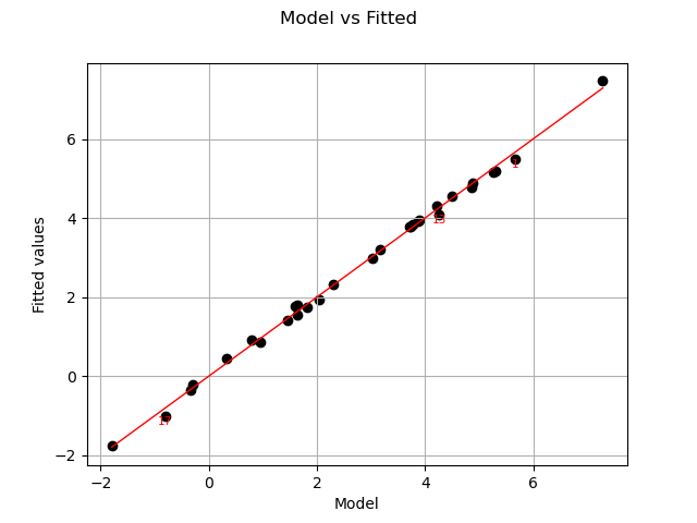
The previous figure seems to indicate that the linearity hypothesis is accurate.

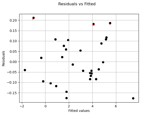
Residuals can be plotted against the fitted values.

graph = analysis.drawResidualsVsFitted()
view = viewer.View(graph)

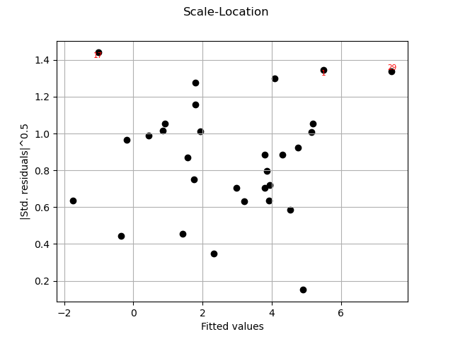
graph = analysis.drawScaleLocation()
view = viewer.View(graph)

graph = analysis.drawQQplot()
view = viewer.View(graph)

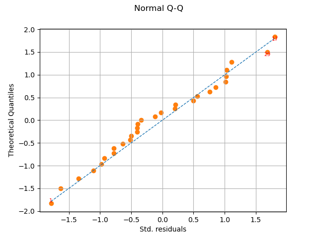
In this case, the two distributions are very close: there is no obvious outlier.

Cook’s distance measures the impact of every individual data point on the linear regression, and can be plotted as follows:

graph = analysis.drawCookDistance()
view = viewer.View(graph)

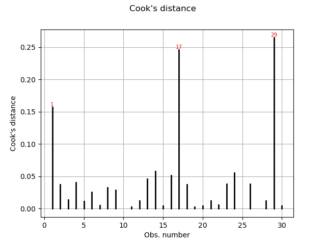
This graph shows us the index of the points with disproportionate influence.

One of the components of the computation of Cook’s distance at a given point is that point’s leverage. High-leverage points are far from their closest neighbors, so the fitted linear regression model must pass close to them.

# sphinx_gallery_thumbnail_number = 6
graph = analysis.drawResidualsVsLeverages()
view = viewer.View(graph)

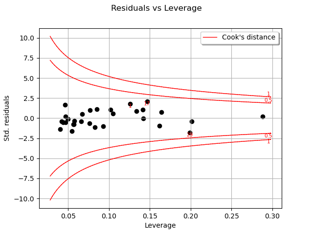
In this case, there seem to be no obvious influential outlier characterized by large leverage and residual values.

Similarly, we can also plot Cook’s distances as a function of the sample leverages:

graph = analysis.drawCookVsLeverages()
view = viewer.View(graph)

Finally, we give the intervals for each estimated coefficient (95% confidence interval):

alpha = 0.95
interval = analysis.getCoefficientsConfidenceInterval(alpha)
print("confidence intervals with level=%1.2f: " % (alpha))
print("%s" % (interval))

confidence intervals with level=0.95:
[2.99855, 3.01079]
[1.99374, 2.00616]
[-1.00395, -0.991707]