Taylor approximations¶

In this example we build a local approximation of a model using the Taylor decomposition with the LinearTaylor class.

We consider the function $\vect{h} : \Rset^2 \rightarrow \Rset^2$ defined by:

$\vect{h}(\vect{x}) = \Tr{\left( \cos(x_1 + x_2), (x_2 + 1) e^{x_1 - 2 x_2} \right)}.$

for any $\vect{x} \in \Rset^2$ . The metamodel $\widehat{\vect{h}}$ is an approximation of the model $\vect{h}$ :

$\vect{y} \approx \widehat{\vect{h}}(\vect{x})$

for any $\vect{x} \in \Rset^2$ . We note $h_k$ , $k=1, 2$ the marginal outputs In this example, we consider two different approximations:

the first order Taylor expansion,
the second order Taylor expansion.

import openturns as ot
import openturns.viewer as viewer

ot.Log.Show(ot.Log.NONE)

Define the model¶

Prepare some data.

formulas = ["cos(x1 + x2)", "(x2 + 1) * exp(x1 - 2 * x2)"]
model = ot.SymbolicFunction(["x1", "x2"], formulas)

Center of the approximation.

x0 = [-0.4, -0.4]

Drawing bounds.

a = -0.4
b = 0.0

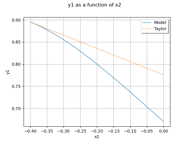
First order Taylor expansion¶

Let $\vect{x}_0 \in \Rset^2$ be a reference point where the linear approximation is evaluated. The first order Taylor expansion of the output marginal $h_k$ is:

$\widehat{h_k}(\vect{x}) = h_k(\vect{x}_0) + \sum_{i=1}^{2} \frac{\partial h_k}{\partial x_i}(\vect{x}_0) \left(x_i - x_{0,i} \right)$

for any $\vect{x} \in \Rset^2$ .

Create a linear (first-order) Taylor approximation.

algo = ot.LinearTaylor(x0, model)
algo.run()
responseSurface = algo.getMetaModel()

Plot the second output of our model with $x_1=x_{0,1}$ .

graph = ot.ParametricFunction(model, [0], [x0[1]]).getMarginal(1).draw(a, b)
graph.setLegends(["Model"])
curve = (
    ot.ParametricFunction(responseSurface, [0], [x0[1]])
    .getMarginal(1)
    .draw(a, b)
    .getDrawable(0)
)
curve.setLegend("Taylor")
curve.setLineStyle("dashed")
graph.add(curve)
graph.setLegendPosition("upper right")
view = viewer.View(graph)

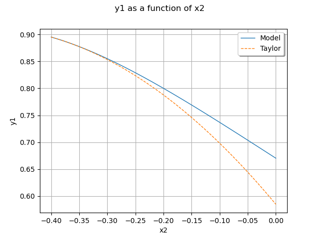
Second order Taylor expansion¶

Let $\vect{x}_0 \in \Rset^2$ be a reference point where the quadratic approximation is evaluated. The second order Taylor expansion of the output marginal $h_k$ is:

$\widehat{h_k}(\vect{x}) = h_k(\vect{x}_0) + \sum_{i=1}^{2} \frac{\partial h_k}{\partial x_i}(\vect{x}_0) \left(x_i - x_{0,i} \right) + \frac{1}{2} \sum_{i,j=1}^{2} \frac{\partial^2 h_k}{\partial x_i \partial x_j}(\vect{x}_0) \left(x_i - x_{0,i} \right) \left(x_j - x_{0,j} \right)$

for any $\vect{x} \in \Rset^2$ .

Create a quadratic (second-order) Taylor approximation.

algo = ot.QuadraticTaylor(x0, model)
algo.run()
responseSurface = algo.getMetaModel()

Plot second output of our model with $x_1=x_{0,1}$ .

graph = ot.ParametricFunction(model, [0], [x0[1]]).getMarginal(1).draw(a, b)
graph.setLegends(["Model"])
curve = (
    ot.ParametricFunction(responseSurface, [0], [x0[1]])
    .getMarginal(1)
    .draw(a, b)
    .getDrawable(0)
)
curve.setLegend("Taylor")
curve.setLineStyle("dashed")
graph.add(curve)
graph.setLegendPosition("upper right")
view = viewer.View(graph)

view.ShowAll()

OpenTURNS

An Open source initiative for the Treatment of Uncertainties, Risks'N Statistics

Table of Contents

Previous topic

Next topic

This Page

Taylor approximations¶

Define the model¶

First order Taylor expansion¶

Second order Taylor expansion¶