Advanced Kriging

In this example we will build a metamodel using Gaussian process regression of the function.

We will choose the number of learning points, the basis and the covariance model.

import openturns as ot
from openturns.viewer import View
import numpy as np
import matplotlib.pyplot as plt
import openturns.viewer as viewer

ot.Log.Show(ot.Log.NONE)

Generate design of experiments

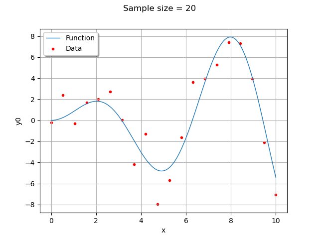
We create training samples from the function . We can change their number and distribution in the range. If the with_error boolean is True, then the data is computed by adding a Gaussian noise to the function values.

dim = 1
xmin = 0
xmax = 10
n_pt = 20  # number of initial points
with_error = True  # whether to use generation with error

ref_func_with_error = ot.SymbolicFunction(["x", "eps"], ["x * sin(x) + eps"])
ref_func = ot.ParametricFunction(ref_func_with_error, [1], [0.0])
x = np.vstack(np.linspace(xmin, xmax, n_pt))
ot.RandomGenerator.SetSeed(1235)
eps = ot.Normal(0, 1.5).getSample(n_pt)
X = ot.Sample(n_pt, 2)
X[:, 0] = x
X[:, 1] = eps
if with_error:
    y = np.array(ref_func_with_error(X))
else:
    y = np.array(ref_func(x))

graph = ref_func.draw(xmin, xmax, 200)
cloud = ot.Cloud(x, y)
cloud.setColor("red")
cloud.setPointStyle("bullet")
graph.add(cloud)
graph.setLegends(["Function", "Data"])
graph.setLegendPosition("upper left")
graph.setTitle("Sample size = %d" % (n_pt))
view = viewer.View(graph)

Create the Kriging algorithm

# 1. Basis
ot.ResourceMap.SetAsBool(
    "GeneralLinearModelAlgorithm-UseAnalyticalAmplitudeEstimate", True
)
basis = ot.ConstantBasisFactory(dim).build()
print(basis)

# 2. Covariance model
cov = ot.MaternModel([1.0], [2.5], 1.5)
print(cov)

# 3. Kriging algorithm
algokriging = ot.KrigingAlgorithm(x, y, cov, basis)

# error measure
# algokriging.setNoise([5*1e-1]*n_pt)

# 4. Optimization
# algokriging.setOptimizationAlgorithm(ot.NLopt('GN_DIRECT'))
lhsExperiment = ot.LHSExperiment(ot.Uniform(1e-1, 1e2), 50)
algokriging.setOptimizationAlgorithm(ot.MultiStart(ot.TNC(), lhsExperiment.generate()))
algokriging.setOptimizationBounds(ot.Interval([0.1], [1e2]))

# if we choose not to optimize parameters
# algokriging.setOptimizeParameters(False)

# 5. Run the algorithm
algokriging.run()

Basis( [class=LinearEvaluation name=Unnamed center=[0] constant=[1] linear=[[ 0 ]]] )
MaternModel(scale=[1], amplitude=[2.5], nu=1.5)

Results

Get some results

krigingResult = algokriging.getResult()
print("residual = ", krigingResult.getResiduals())
print("R2 = ", krigingResult.getRelativeErrors())
print("Optimal scale= {}".format(krigingResult.getCovarianceModel().getScale()))
print(
    "Optimal amplitude = {}".format(krigingResult.getCovarianceModel().getAmplitude())
)
print("Optimal trend coefficients = {}".format(krigingResult.getTrendCoefficients()))

residual =  [5.39875e-16]
R2 =  [2.99965e-31]
Optimal scale= [0.818671]
Optimal amplitude = [4.51225]
Optimal trend coefficients = [-0.115697]

Get the metamodel

krigingMeta = krigingResult.getMetaModel()

n_pts_plot = 1000
x_plot = np.vstack(np.linspace(xmin, xmax, n_pts_plot))
fig, [ax1, ax2] = plt.subplots(1, 2, figsize=(12, 6))

# On the left, the function
graph = ref_func.draw(xmin, xmax, n_pts_plot)
graph.setLegends(["Function"])
graphKriging = krigingMeta.draw(xmin, xmax, n_pts_plot)
graphKriging.setColors(["green"])
graphKriging.setLegends(["Kriging"])
graph.add(graphKriging)
cloud = ot.Cloud(x, y)
cloud.setColor("red")
cloud.setLegend("Data")
graph.add(cloud)
graph.setLegendPosition("upper left")
View(graph, axes=[ax1])

# On the right, the conditional Kriging variance
graph = ot.Graph("", "x", "Conditional Kriging variance", True, "")
# Sample for the data
sample = ot.Sample(n_pt, 2)
sample[:, 0] = x
cloud = ot.Cloud(sample)
cloud.setColor("red")
graph.add(cloud)
# Sample for the variance
sample = ot.Sample(n_pts_plot, 2)
sample[:, 0] = x_plot
variance = [[krigingResult.getConditionalCovariance(xx)[0, 0]] for xx in x_plot]
sample[:, 1] = variance
curve = ot.Curve(sample)
curve.setColor("green")
graph.add(curve)
View(graph, axes=[ax2])

fig.suptitle("Kriging result")

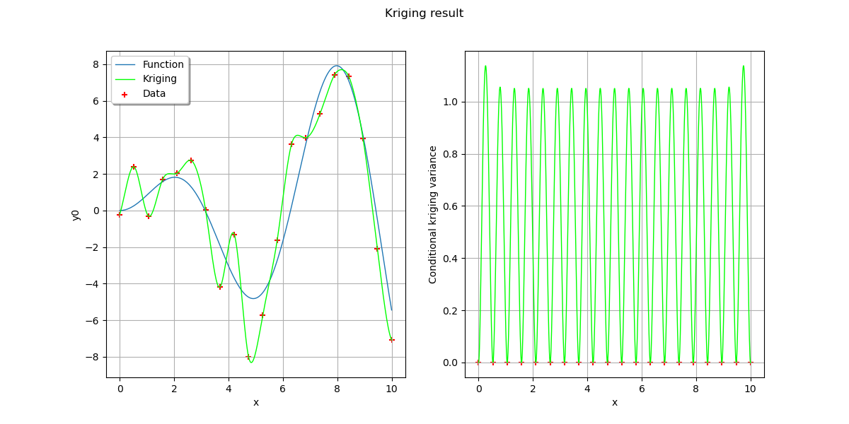
Text(0.5, 0.98, 'Kriging result')

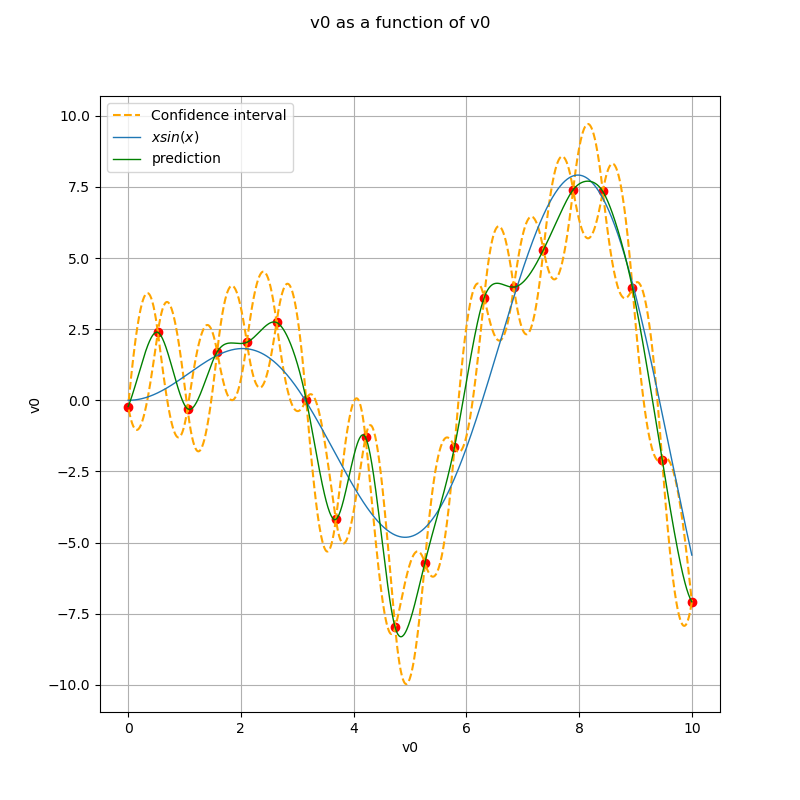
Display the confidence interval

level = 0.95
quantile = ot.Normal().computeQuantile((1 - level) / 2)[0]
borne_sup = krigingMeta(x_plot) + quantile * np.sqrt(variance)
borne_inf = krigingMeta(x_plot) - quantile * np.sqrt(variance)

fig, ax = plt.subplots(figsize=(8, 8))
ax.plot(x, y, ("ro"))
ax.plot(x_plot, borne_sup, "--", color="orange", label="Confidence interval")
ax.plot(x_plot, borne_inf, "--", color="orange")
graph_ref_func = ref_func.draw(xmin, xmax, n_pts_plot)
graph_krigingMeta = krigingMeta.draw(xmin, xmax, n_pts_plot)
for graph in [graph_ref_func, graph_krigingMeta]:
    graph.setTitle("")
View(graph_ref_func, axes=[ax], plot_kw={"label": "$x sin(x)$"})
View(
    graph_krigingMeta,
    plot_kw={"color": "green", "label": "prediction"},
    axes=[ax],
)
legend = ax.legend()
ax.autoscale()

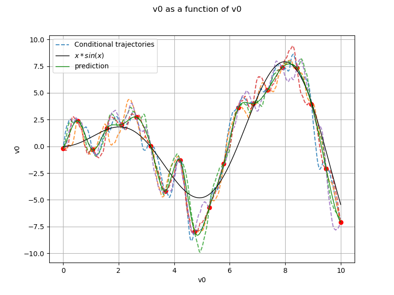
Generate conditional trajectories

Support for trajectories with training samples removed

values = np.linspace(0, 10, 500)
for xx in x:
    if len(np.argwhere(values == xx)) == 1:
        values = np.delete(values, np.argwhere(values == xx)[0, 0])

Conditional Gaussian process

krv = ot.KrigingRandomVector(krigingResult, np.vstack(values))
krv_sample = krv.getSample(5)

x_plot = np.vstack(np.linspace(xmin, xmax, n_pts_plot))
fig, ax = plt.subplots(figsize=(8, 6))
ax.plot(x, y, ("ro"))
for i in range(krv_sample.getSize()):
    if i == 0:
        ax.plot(
            values, krv_sample[i, :], "--", alpha=0.8, label="Conditional trajectories"
        )
    else:
        ax.plot(values, krv_sample[i, :], "--", alpha=0.8)
View(
    graph_ref_func,
    axes=[ax],
    plot_kw={"color": "black", "label": "$x*sin(x)$"},
)
View(
    graph_krigingMeta,
    axes=[ax],
    plot_kw={"color": "green", "label": "prediction"},
)
legend = ax.legend()
ax.autoscale()

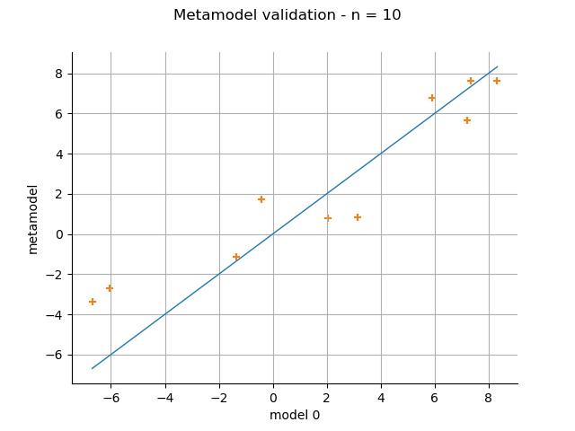
Validation

n_valid = 10
x_valid = ot.Uniform(xmin, xmax).getSample(n_valid)
X_valid = ot.Sample(x_valid)
if with_error:
    X_valid.stack(ot.Normal(0.0, 1.5).getSample(n_valid))
    y_valid = np.array(ref_func_with_error(X_valid))
else:
    y_valid = np.array(ref_func(X_valid))

metamodelPredictions = krigingMeta(x_valid)
validation = ot.MetaModelValidation(y_valid, metamodelPredictions)
validation.computeR2Score()

class=Point name=Unnamed dimension=1 values=[0.861246]

graph = validation.drawValidation()
view = viewer.View(graph)

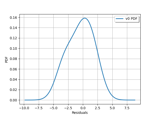
graph = validation.getResidualDistribution().drawPDF()
graph.setXTitle("Residuals")
view = viewer.View(graph)

Nugget effect

Let us try again, but this time we optimize the nugget effect.

cov.activateNuggetFactor(True)

We have to run the optimization algorithm again.

algokriging_nugget = ot.KrigingAlgorithm(x, y, cov, basis)
algokriging_nugget.setOptimizationAlgorithm(ot.NLopt("GN_DIRECT"))
algokriging_nugget.run()

We get the results and the metamodel.

krigingResult_nugget = algokriging_nugget.getResult()
print("residual = ", krigingResult_nugget.getResiduals())
print("R2 = ", krigingResult_nugget.getRelativeErrors())
print("Optimal scale= {}".format(krigingResult_nugget.getCovarianceModel().getScale()))
print(
    "Optimal amplitude = {}".format(
        krigingResult_nugget.getCovarianceModel().getAmplitude()
    )
)
print(
    "Optimal trend coefficients = {}".format(
        krigingResult_nugget.getTrendCoefficients()
    )
)

residual =  [6.52848e-16]
R2 =  [4.3864e-31]
Optimal scale= [1.15712]
Optimal amplitude = [4.67517]
Optimal trend coefficients = [-0.350133]

krigingMeta_nugget = krigingResult_nugget.getMetaModel()
variance = [[krigingResult_nugget.getConditionalCovariance(xx)[0, 0]] for xx in x_plot]

Plot the confidence interval again. Note that this time, it always contains the true value of the function.

# sphinx_gallery_thumbnail_number = 7
borne_sup_nugget = krigingMeta_nugget(x_plot) + quantile * np.sqrt(variance)
borne_inf_nugget = krigingMeta_nugget(x_plot) - quantile * np.sqrt(variance)

fig, ax = plt.subplots(figsize=(8, 8))
ax.plot(x, y, ("ro"))
ax.plot(
    x_plot,
    borne_sup_nugget,
    "--",
    color="orange",
    label="Confidence interval with nugget",
)
ax.plot(x_plot, borne_inf_nugget, "--", color="orange")
graph_krigingMeta_nugget = krigingMeta_nugget.draw(xmin, xmax, n_pts_plot)
graph_krigingMeta_nugget.setTitle("")
View(graph_ref_func, axes=[ax], plot_kw={"label": "$x sin(x)$"})
View(
    graph_krigingMeta_nugget,
    plot_kw={"color": "green", "label": "prediction with nugget"},
    axes=[ax],
)
View(
    graph_krigingMeta,
    plot_kw={
        "color": "green",
        "linestyle": "dotted",
        "label": "prediction without nugget",
    },
    axes=[ax],
)
legend = ax.legend()
ax.autoscale()

plt.show()

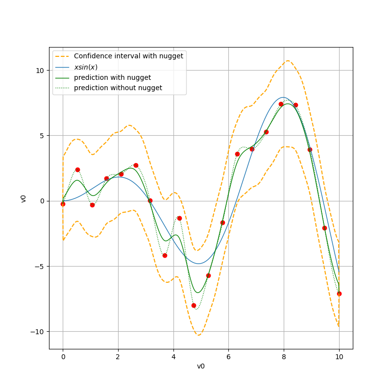
We validate the model with the nugget effect: its predictivity factor is slightly improved.

validation_nugget = ot.MetaModelValidation(y_valid, krigingMeta_nugget(x_valid))
print("R2 score with nugget: ", validation_nugget.computeR2Score())
print("R2 score without nugget: ", validation.computeR2Score())

R2 score with nugget:  [0.884249]
R2 score without nugget:  [0.861246]

Reset default settings

ot.ResourceMap.Reload()