GaussianProcessRegression¶

(Source code, png)

class GaussianProcessRegression(*args)¶

Gaussian process regression algorithm.

Warning

This class is experimental and likely to be modified in future releases. To use it, import the openturns.experimental submodule.

Refer to Kriging.

Available constructors:

GaussianProcessRegression(gprFitterResult)

GaussianProcessRegression(inputSample, outputSample, covarianceModel, trendFunction)

Parameters:

gprFitterResultGaussianProcessFitterResult: Result class
inputSample, outputSample2-d sequence of float: The samples $(\vect{x}_k)_{1 \leq k \leq \sampleSize} \in \Rset^{\inputDim}$ and $(\vect{y}_k)_{1 \leq k \leq \sampleSize}\in \Rset^{\outputDim}$ upon which the meta-model is built.
covarianceModelCovarianceModel
covarianceModelCovarianceModel: Covariance model used for the underlying Gaussian process assumption.
trendFunctionFunction: A trend function

Methods

`BuildDistribution`(inputSample)	Recover the distribution, with metamodel performance in mind.
`getClassName`()	Accessor to the object's name.
`getDistribution`()	Accessor to the joint probability density function of the physical input vector.
`getInputSample`()	Accessor to the input sample.
`getName`()	Accessor to the object's name.
`getOutputSample`()	Accessor to the output sample.
`getResult`()	Get the results of the metamodel computation.
`getWeights`()	Return the weights of the input sample.
`hasName`()	Test if the object is named.
`run`()	Compute the response surface.
`setDistribution`(distribution)	Accessor to the joint probability density function of the physical input vector.
`setName`(name)	Accessor to the object's name.

Notes

We suppose we have a sample $(\vect{x}_k, \vect{y}_k)_{1 \leq k \leq \sampleSize}$ where $\vect{y}_k = \cM(\vect{x}_k)$ for all k, with $\cM:\Rset^{\inputDim} \mapsto \Rset^{\outputDim}$ the model. The class allows making a gaussian process interpolating on the input samples.

Within the first constructor, we suppose all gaussian process parameters (the trend coefficients $\beta_j^l$ , the scale $\vect{\theta}$ and the amplitude $\vect{\sigma}$ ) already calibrated and the objective is to condionning this process (the gaussian process to become interpolating over the dataset)

Within the second constructor, we assume covariance model already calibrated. A gaussian process is fitted using GaussianProcessFitter and the sample $(\vect{y}_k)_{1 \leq k \leq \sampleSize}$ is considered as the trace of a this gaussian process $\vect{Y}(\omega, \vect{x})$ on $(\vect{x}_k)_{1 \leq k \leq \sampleSize}$ .

The Gaussian process $\vect{Y}(\omega, \vect{x})$ is defined by:

(1)¶ $\vect{Y}(\omega, \vect{x}) = \vect{\mu}(\vect{x}) + W(\omega, \vect{x})$

where:

$\vect{\mu}(\vect{x}) = \left( \begin{array}{l} \mu_1(\vect{x}) \\ \dots \\ \mu_p(\vect{x}) \end{array} \right)$

with $\mu_l(\vect{x}) = \sum_{j=1}^{n_l} \beta_j^l \varphi_j^\ell(\vect{x})$ and $\varphi_j^\ell: \Rset^{\inputDim} \rightarrow \Rset$ the trend functions.

$W$ is a Gaussian process of dimension p with zero mean and covariance function $C = C(\vect{\theta}, \vect{\sigma}, \mat{R}, \vect{\lambda})$ (see CovarianceModel for the notations).

The Gaussian Process Regression meta model $\tilde{\cM}$ is defined by:

$\tilde{\cM}(\vect{x}) = \vect{\mu}(\vect{x}) + \Expect{\vect{Y}(\omega, \vect{x})\, | \, \cC}$

where $\cC$ is the condition $\vect{Y}(\omega, \vect{x}_k) = \vect{y}_k$ for each $k \in [1, \sampleSize]$ .

(1) writes:

$\tilde{\cM}(\vect{x}) = \vect{\mu}(\vect{x}) + \Cov{\vect{Y}(\omega, \vect{x}), (\vect{Y}(\omega, \vect{x}_1), \dots, \vect{Y}(\omega, \vect{x}_{\sampleSize}))} \vect{\gamma}$

where $\Cov{\vect{Y}(\omega, \vect{x}), (\vect{Y}(\omega, \vect{x}_1), \dots, \vect{Y}(\omega, \vect{x}_{\sampleSize}))} = \left( \mat{C}( \vect{x}, \vect{x}_1) | \dots | \mat{C}( \vect{x}, \vect{x}_{\sampleSize}) \right)$ is a matrix in $\cM_{\inputDim,\sampleSize \times \outputDim}(\Rset)$ and $\vect{\gamma} = \mat{C}^{-1}(\vect{y}-\vect{m})$ .

Examples

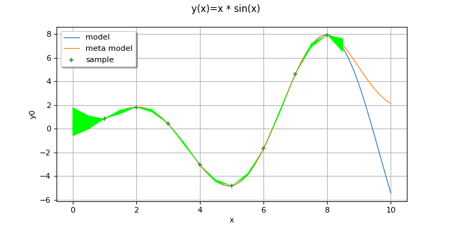
Create the model $\cM: \Rset \mapsto \Rset$ and the samples:

>>> import openturns as ot
>>> import openturns.experimental as otexp
>>> g = ot.SymbolicFunction(['x'],  ['x * sin(x)'])
>>> sampleX = [[1.0], [2.0], [3.0], [4.0], [5.0], [6.0], [7.0], [8.0]]
>>> sampleY = g(sampleX)

Create the algorithm:

>>> basis = ot.Basis([ot.SymbolicFunction(['x'], ['x']), ot.SymbolicFunction(['x'], ['x^2'])])
>>> covarianceModel = ot.SquaredExponential([1.0])
>>> covarianceModel.setActiveParameter([])
>>> fit_algo = otexp.GaussianProcessFitter(sampleX, sampleY, covarianceModel, basis)
>>> fit_algo.run()

Get the resulting meta model:

>>> fit_result = fit_algo.getResult()
>>> algo = otexp.GaussianProcessRegression(fit_result)
>>> algo.run()
>>> result = algo.getResult()
>>> metamodel = result.getMetaModel()

__init__(*args)¶

static BuildDistribution(inputSample)¶

Recover the distribution, with metamodel performance in mind.

For each marginal, find the best 1-d continuous parametric model else fallback to the use of a nonparametric one.

The selection is done as follow:

We start with a list of all parametric models (all factories)

For each model, we estimate its parameters if feasible.

We check then if model is valid, ie if its Kolmogorov score exceeds a threshold fixed in the MetaModelAlgorithm-PValueThreshold ResourceMap key. Default value is 5%

We sort all valid models and return the one with the optimal criterion.

For the last step, the criterion might be BIC, AIC or AICC. The specification of the criterion is done through the MetaModelAlgorithm-ModelSelectionCriterion ResourceMap key. Default value is fixed to BIC. Note that if there is no valid candidate, we estimate a non-parametric model (KernelSmoothing or Histogram). The MetaModelAlgorithm-NonParametricModel ResourceMap key allows selecting the preferred one. Default value is Histogram

One each marginal is estimated, we use the Spearman independence test on each component pair to decide whether an independent copula. In case of non independence, we rely on a NormalCopula.

Parameters:

sampleSample: Input sample.

Returns:

distributionDistribution: Input distribution.

getClassName()¶

Accessor to the object’s name.

Returns:

class_namestr: The object class name (object.__class__.__name__).

getDistribution()¶

Accessor to the joint probability density function of the physical input vector.

Returns:

distributionDistribution: Joint probability density function of the physical input vector.

getInputSample()¶

Accessor to the input sample.

Returns:

inputSampleSample: Input sample of a model evaluated apart.

getName()¶

Accessor to the object’s name.

Returns:

namestr: The name of the object.

getOutputSample()¶

Accessor to the output sample.

Returns:

outputSampleSample: Output sample of a model evaluated apart.

getResult()¶

Get the results of the metamodel computation.

Returns:

resultGaussianProcessRegressionResult: Structure containing all the results obtained after computation and created by the method run().

getWeights()¶

Return the weights of the input sample.

Returns:

weightssequence of float: The weights of the points in the input sample.

hasName()¶

Test if the object is named.

Returns:

hasNamebool: True if the name is not empty.

run()¶

Compute the response surface.

Notes

It computes the kriging response surface and creates a GaussianProcessRegressionResult structure containing all the results.

setDistribution(distribution)¶

Accessor to the joint probability density function of the physical input vector.

Parameters:

distributionDistribution: Joint probability density function of the physical input vector.

setName(name)¶

Accessor to the object’s name.

Parameters:

namestr: The name of the object.

Examples using the class¶

Gaussian Process Regression : cantilever beam model

Gaussian Process Regression : quick-start

Sequentially adding new points to a Kriging

OpenTURNS

An Open source initiative for the Treatment of Uncertainties, Risks'N Statistics

Table of Contents

Previous topic

Next topic

This Page

GaussianProcessRegression¶

Examples using the class¶