Bayesian calibration of the flooding model

Abstract

The goal of this example is to present the statistical hypotheses of the bayesian calibration of the flooding model.

Parameters to calibrate

The vector of parameters to calibrate is:

The variables to calibrate are and are set to the following values:

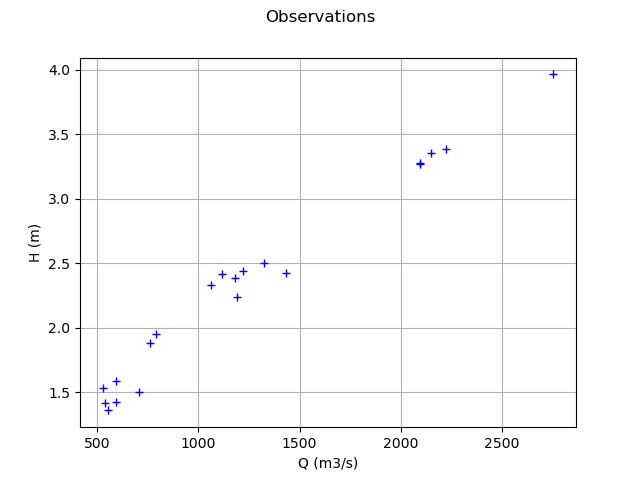
Observations

In this section, we describe the statistical model associated with the observations. The errors of the water heights are associated with a gaussian distribution with a zero mean and a standard variation equal to:

Therefore, the observed water heights are:

for where

and we make the hypothesis that the observation errors are independent. We consider a sample size equal to:

The observations are the couples , i.e. each observation is a couple made of the flowrate and the corresponding river height.

Analysis

In this model, the variables and are not identifiables, since only the difference matters. Hence, calibrating this model requires some regularization.

Generate the observations

import numpy as np
import openturns as ot
ot.Log.Show(ot.Log.NONE)
import openturns.viewer as viewer

A basic implementation of the probabilistic model is available in the usecases module :

from openturns.usecases import flood_model as flood_model
fm = flood_model.FloodModel()

We define the model which has 4 inputs and one output H.

The nonlinear least squares does not take into account for bounds in the parameters. Therefore, we ensure that the output is computed whatever the inputs. The model fails into two situations:

• if ,

• if .

In these cases, we return an infinite number.

def functionFlooding(X) :
    L = 5.0e3
    B = 300.0
    Q, K_s, Z_v, Z_m = X
    alpha = (Z_m - Z_v)/L
    if alpha < 0.0 or K_s <= 0.0:
        H = np.inf
    else:
        H = (Q/(K_s*B*np.sqrt(alpha)))**(3.0/5.0)
    return [H]

g = ot.PythonFunction(4, 1, functionFlooding)
g = ot.MemoizeFunction(g)
g.setOutputDescription(["H (m)"])

We load the input distribution for .

Q = fm.Q

Set the parameters to be calibrated.

K_s = ot.Dirac(30.0)
Z_v = ot.Dirac(50.0)
Z_m = ot.Dirac(55.0)
K_s.setDescription(["Ks (m^(1/3)/s)"])
Z_v.setDescription(["Zv (m)"])
Z_m.setDescription(["Zm (m)"])

We create the joint input distribution.

inputRandomVector = ot.ComposedDistribution([Q, K_s, Z_v, Z_m])

Create a Monte-Carlo sample of the output H.

nbobs = 20
inputSample = inputRandomVector.getSample(nbobs)
outputH = g(inputSample)

Generate the observation noise and add it to the output of the model.

sigmaObservationNoiseH = 0.1 # (m)
noiseH = ot.Normal(0.,sigmaObservationNoiseH)
ot.RandomGenerator.SetSeed(0)
sampleNoiseH = noiseH.getSample(nbobs)
Hobs = outputH + sampleNoiseH

Plot the Y observations versus the X observations.

Qobs = inputSample[:,0]

graph = ot.Graph("Observations","Q (m3/s)","H (m)",True)
cloud = ot.Cloud(Qobs,Hobs)
graph.add(cloud)
view = viewer.View(graph)

Setting the calibration parameters

Define the parametric model that associates each observation and values of the parameters to the parameters of the distribution of the corresponding observation: here

def fullModelPy(X):
    Q, K_s, Z_v, Z_m = X
    H = g(X)[0]
    sigmaH = 0.5 # (m^2) The standard deviation of the observation error.
    return [H,sigmaH]

fullModel = ot.PythonFunction(4, 2, fullModelPy)
model = ot.ParametricFunction(fullModel, [0], Qobs[0])
model

ParametricEvaluation(class=PythonEvaluation name=OpenTURNSPythonFunction, parameters positions=[0], parameters=[x0 : 2752.94], input positions=[1,2,3])

Define the value of the reference values of the parameter. In the bayesian framework, this is called the mean of the prior gaussian distribution. In the data assimilation framework, this is called the background.

KsInitial = 20.
ZvInitial = 49.
ZmInitial = 51.
parameterPriorMean = ot.Point([KsInitial,ZvInitial,ZmInitial])
paramDim = parameterPriorMean.getDimension()

Define the covariance matrix of the parameters to calibrate.

sigmaKs = 5.
sigmaZv = 1.
sigmaZm = 1.

parameterPriorCovariance = ot.CovarianceMatrix(paramDim)
parameterPriorCovariance[0,0] = sigmaKs**2
parameterPriorCovariance[1,1] = sigmaZv**2
parameterPriorCovariance[2,2] = sigmaZm**2
parameterPriorCovariance

[[ 25 0 0 ]
[ 0 1 0 ]
[ 0 0 1 ]]

Define the the prior distribution of the parameter

prior = ot.Normal(parameterPriorMean,parameterPriorCovariance)
prior.setDescription(['Ks', 'Zv', 'Zm'])
prior

Normal(mu = [20,49,51], sigma = [5,1,1], R = [[ 1 0 0 ]
[ 0 1 0 ]
[ 0 0 1 ]])

Define the distribution of observations conditional on model predictions.

Note that its parameter dimension is the one of , so the model must be adjusted accordingly. In other words, the input argument of the setParameter method of the conditional distribution must be equal to the dimension of the output of the model. Hence, we do not have to set the actual parameters: only the type of distribution is used.

conditional = ot.Normal()
conditional

Normal(mu = 0, sigma = 1)

Proposal distribution: uniform.

proposal = [ot.Uniform(-5., 5.),ot.Uniform(-1., 1.),ot.Uniform(-1., 1.)]
proposal

Out:

[class=Uniform name=Uniform dimension=1 a=-5 b=5, class=Uniform name=Uniform dimension=1 a=-1 b=1, class=Uniform name=Uniform dimension=1 a=-1 b=1]

Test the MCMC sampler

The MCMC sampler essentially computes the log-likelihood of the parameters.

mymcmc = ot.MCMC(prior, conditional, model, Qobs, Hobs, parameterPriorMean)

mymcmc.computeLogLikelihood(parameterPriorMean)

Out:

-118.8899132627309

Test the Metropolis-Hastings sampler

• Creation of the Random Walk Metropolis-Hastings (RWMH) sampler.

initialState = parameterPriorMean

RWMHsampler = ot.RandomWalkMetropolisHastings(
    prior, conditional, model, Qobs, Hobs, initialState, proposal)

Tuning of the RWMH algorithm.

Strategy of calibration for the random walk (trivial example: default).

strategy = ot.CalibrationStrategyCollection(paramDim)
RWMHsampler.setCalibrationStrategyPerComponent(strategy)

Other parameters.

RWMHsampler.setVerbose(True)
RWMHsampler.setThinning(1)
RWMHsampler.setBurnIn(200)

Generate a sample from the posterior distribution of the parameters theta.

sampleSize = 1000
sample = RWMHsampler.getSample(sampleSize)

Look at the acceptance rate (basic checking of the efficiency of the tuning; value close to 0.2 usually recommended).

RWMHsampler.getAcceptanceRate()

[0.546667,0.619167,0.604167]

Build the distribution of the posterior by kernel smoothing.

kernel = ot.KernelSmoothing()
posterior = kernel.build(sample)

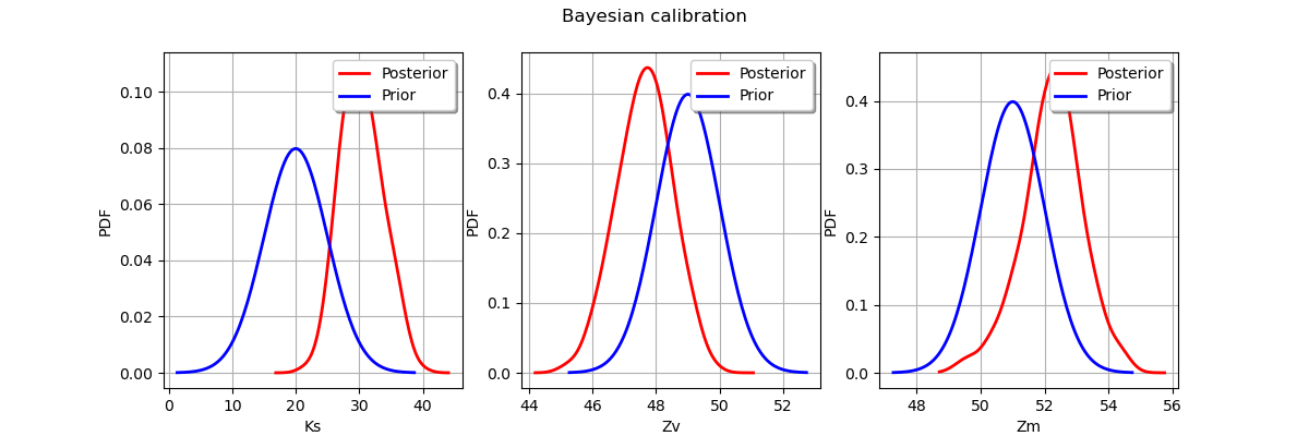
Display prior vs posterior for each parameter.

from openturns.viewer import View
import pylab as pl

fig = pl.figure(figsize=(12, 4))

for parameter_index in range(paramDim):
    graph = posterior.getMarginal(parameter_index).drawPDF()
    priorGraph = prior.getMarginal(parameter_index).drawPDF()
    priorGraph.setColors(['blue'])
    graph.add(priorGraph)
    graph.setLegends(['Posterior', 'Prior'])
    ax = fig.add_subplot(1, paramDim, parameter_index+1)
    _ = ot.viewer.View(graph, figure=fig, axes=[ax])

_ = fig.suptitle("Bayesian calibration")