Mixture of experts

In this example we are going to approximate a piece wise continuous function using an expert mixture of metamodels.

The metamodels will be represented by the family of :

where the N classes are defined by the classifier.

Using the supervised mode the classifier partitions the input and output space at once:

The classifier is MixtureClassifier based on a MixtureDistribution defined as:

The rule to assign a point to a class is defined as follows: is assigned to the class .

The grade of with respect to the class is .

from __future__ import print_function
import openturns as ot
from matplotlib import pyplot as plt
import openturns.viewer as viewer
from matplotlib import pylab as plt
from openturns.viewer import View
import numpy as np
ot.Log.Show(ot.Log.NONE)

dimension = 1

# Define the piecewise model we want to rebuild
def piecewise(X):
    # if x < 0.0:
    #     f = (x+0.75)**2-0.75**2
    # else:
    #     f = 2.0-x**2
    xarray = np.array(X, copy=False)
    return np.piecewise(xarray, [xarray < 0, xarray >= 0], [lambda x: x*(x+1.5), lambda x: 2.0 - x*x])
f = ot.PythonFunction(1, 1, func_sample=piecewise)

Build a metamodel over each segment

degree = 5
samplingSize = 100
enumerateFunction = ot.LinearEnumerateFunction(dimension)
productBasis = ot.OrthogonalProductPolynomialFactory([ot.LegendreFactory()] * dimension, enumerateFunction)
adaptiveStrategy = ot.FixedStrategy(productBasis, enumerateFunction.getStrataCumulatedCardinal(degree))
projectionStrategy = ot.LeastSquaresStrategy(ot.MonteCarloExperiment(samplingSize))

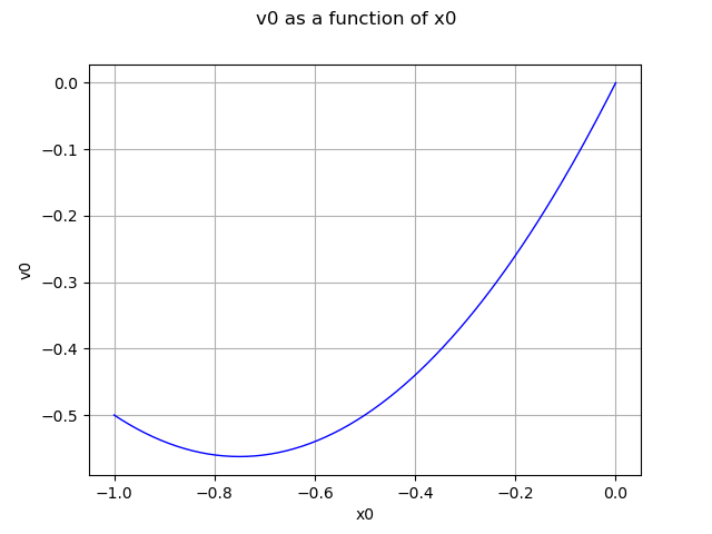
Segment 1: (-1.0; 0.0)

d1 = ot.Uniform(-1.0, 0.0)
fc1 = ot.FunctionalChaosAlgorithm(f, d1, adaptiveStrategy, projectionStrategy)
fc1.run()
mm1 = fc1.getResult().getMetaModel()
graph = mm1.draw(-1.0, -1e-6)
view = viewer.View(graph)

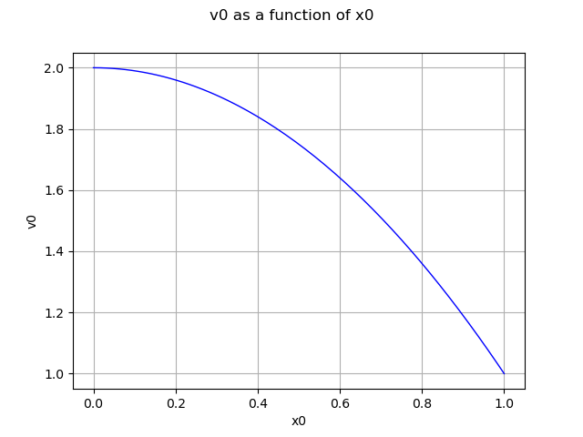
Segment 2: (0.0, 1.0)

d2 = ot.Uniform(0.0, 1.0)
fc2 = ot.FunctionalChaosAlgorithm(f, d2, adaptiveStrategy, projectionStrategy)
fc2.run()
mm2 = fc2.getResult().getMetaModel()
graph = mm2.draw(1e-6,1.0)
view = viewer.View(graph)

Define the mixture

R = ot.CorrelationMatrix(2)
d1 = ot.Normal([-1.0, -1.0], [1.0]*2, R)# segment 1
d2 = ot.Normal([1.0, 1.0], [1.0]*2, R)# segment 2
weights = [1.0]*2
atoms = [d1, d2]
mixture = ot.Mixture(atoms, weights)

Create the classifier based on the mixture

classifier = ot.MixtureClassifier(mixture)

Create local experts using the metamodels

experts = ot.Basis([mm1, mm2])

Create a mixture of experts

evaluation = ot.ExpertMixture(experts, classifier)
moe = ot.Function(evaluation)

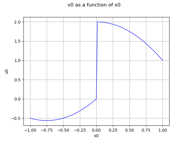
Draw the mixture of experts

graph = moe.draw(-1.0, 1.0)
view = viewer.View(graph)
plt.show()