Note
Click here to download the full example code
Create a process from random vectors and processes
The objective is to create a process defined from a random vector and a process.
We consider the following limit state function, defined as the difference between a degrading resistance  and a time-varying load
  :
:

We propose the following probabilistic model:
-  is the initial resistance, and
  ;
-
;
-  is the deterioration rate of the resistance; it is deterministic;
- is the time-varying stress, which is modeled by a stationary Gaussian process of mean value
is the deterioration rate of the resistance; it is deterministic;
- is the time-varying stress, which is modeled by a stationary Gaussian process of mean value  , standard deviation
  and a squared exponential covariance model;
-
and a squared exponential covariance model;
-  is the time, varying in
 ![[0,T]](../../_images/math/1fae5f98fc818a5b863680eaa5aa290f3df157a4.svg) .
.
First, import the python modules:
from  openturns import *
from openturns.viewer import View
from math import *
1. Create the gaussian process  
Create the mesh which is a regular grid on , with  , by step =1:
b = 0.01
t0 = 0.0
step = 1
tfin = 50
n = round((tfin-t0)/step)
myMesh = RegularGrid(t0, step, n)
Create the squared exeponential covariance model:

where the scale parameter is  and the amplitude
  .
.
l = 10/sqrt(2)
myCovKernel = SquaredExponential([l])
print('cov model = ', myCovKernel)
Out:
cov model = SquaredExponential(scale=[7.07107], amplitude=[1])
Create the gaussian process :
S_proc = GaussianProcess(myCovKernel, myMesh)
2. Create the process  
First, create the random variable , with  and
and  :
:
muR = 5
sigR = 0.3
R = Normal(muR, sigR)
The create the Dirac random variable  :
:
B = Dirac(b)
Then create the process using the  class and the functional basis
  and
and  :
:

with  independent.
const_func = SymbolicFunction(['t'], ['1'])
linear_func = SymbolicFunction(['t'], ['-t'])
myBasis = Basis([const_func, linear_func])

coef = ComposedDistribution([R, B])

R_proc = FunctionalBasisProcess(coef, myBasis, myMesh)
3. Create the process  
First, aggregate both processes into one process of dimension 2: 
myRS_proc = AggregatedProcess([R_proc, S_proc])
Then create the spatial field function that acts only on the values of the process, keeping the mesh unchanged, using the ValueFunction class.
We define the function  on
on  by:
by:

in order to define the spatial field function  that acts on fields, defined by:
![\forall t\in [0,T], g_{dyn}(X(\omega, t), Y(\omega, t)) = X(\omega, t) - Y(\omega, t)](../../_images/math/ec6a79cc22567de945700b0543e47eec71787e99.svg)
g = SymbolicFunction(['x1', 'x2'], ['x1-x2'])
gDyn = ValueFunction(g, myMesh)
Now you have to create the final process  thanks to :
Z_proc = CompositeProcess(gDyn, myRS_proc)
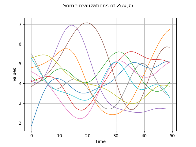
4. Draw some realizations of the process
N=10
sampleZ_proc = Z_proc.getSample(N)
graph = sampleZ_proc.drawMarginal(0)
graph.setTitle(r'Some realizations of $Z(\omega, t)$')

Show(graph)
5. Evaluate the probability that  
We define the domaine ![\mathcal{D} = [2,4]](../../_images/math/63ac0dfc6d33f2cb6ef867f1b477cce1d1de1d23.svg) and the event :
and the event :
domain = Interval([2], [4])
print('D = ', domain)
event = ProcessEvent(Z_proc, domain)
Out:
D = [2, 4]
We use the Monte Carlo sampling to evaluate the probability:
MC_algo = ProbabilitySimulationAlgorithm(event)
MC_algo.setMaximumOuterSampling(1000000)
MC_algo.setBlockSize(100)
MC_algo.setMaximumCoefficientOfVariation(0.01)
MC_algo.run()

result = MC_algo.getResult()

proba = result.getProbabilityEstimate()
print('Probability = ', proba)
variance =  result.getVarianceEstimate()
print('Variance Estimate = ', variance)
IC90_low = proba- result.getConfidenceLength(0.90)/2
IC90_upp = proba + result.getConfidenceLength(0.90)/2
print('IC (90%) = [', IC90_low, ', ', IC90_upp, ']')
Out:
Probability =  0.7551515151515152
Variance Estimate =  5.659164649247292e-05
IC (90%) = [ 0.7427777057653888 ,  0.7675253245376417 ]
Total running time of the script: ( 0 minutes 0.129 seconds)