Axial stressed beam : comparing different methods to estimate a probability

In this example, we compare four methods to estimate the probability in the axial stressed beam example :

• Monte-Carlo simulation,

• FORM,

• directional sampling,

• importance sampling with FORM design point: FORM-IS.

Define the model

from __future__ import print_function

import openturns as ot
import openturns.viewer as viewer
from matplotlib import pylab as plt
ot.Log.Show(ot.Log.NONE)

We load the model from the usecases module :

from openturns.usecases import stressed_beam as stressed_beam
sm = stressed_beam.AxialStressedBeam()

The limit state function is defined in the model field of the data class :

limitStateFunction = sm.model

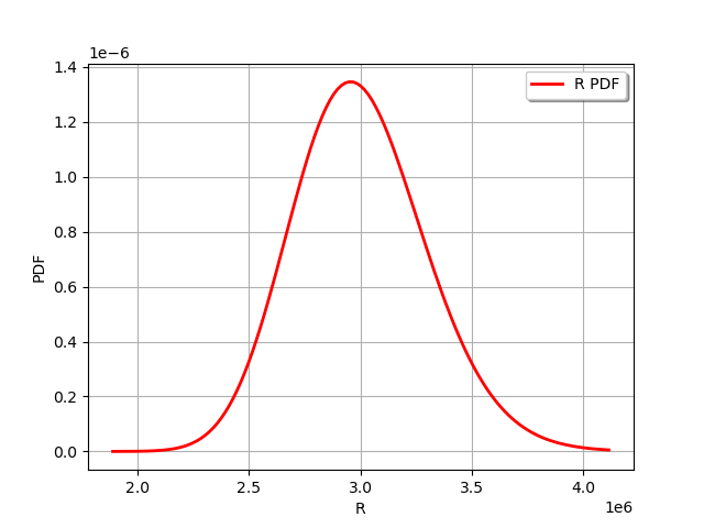
The probabilistic model of the axial stressed beam is defined in the data class. We get the first marginal and draw it :

R_dist = sm.distribution_R
graph = R_dist.drawPDF()
view = viewer.View(graph)

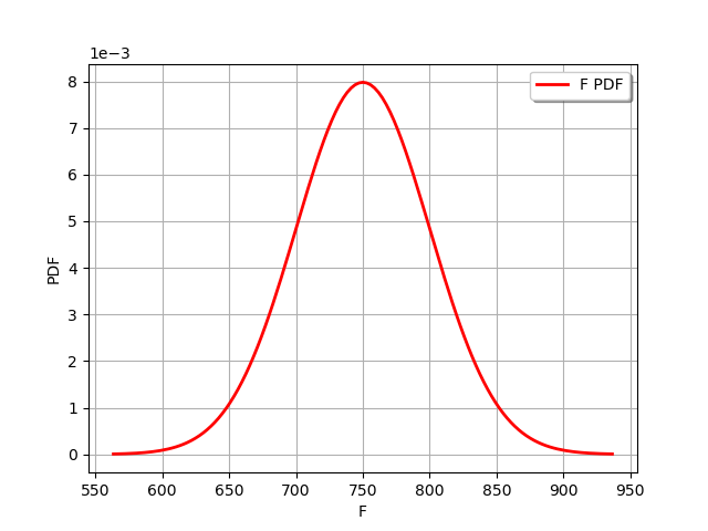
We get the second marginal and draw it :

F_dist = sm.distribution_F
graph = F_dist.drawPDF()
view = viewer.View(graph)

These independent marginals define the joint distribution of the input parameters :

myDistribution = sm.distribution

We create a RandomVector from the Distribution, then a composite random vector. Finally, we create a ThresholdEvent from this RandomVector.

inputRandomVector = ot.RandomVector(myDistribution)
outputRandomVector = ot.CompositeRandomVector(limitStateFunction, inputRandomVector)
myEvent = ot.ThresholdEvent(outputRandomVector, ot.Less(), 0.0)

Using Monte Carlo simulations

cv = 0.05
NbSim = 100000

experiment = ot.MonteCarloExperiment()
algoMC = ot.ProbabilitySimulationAlgorithm(myEvent, experiment)
algoMC.setMaximumOuterSampling(NbSim)
algoMC.setBlockSize(1)
algoMC.setMaximumCoefficientOfVariation(cv)

For statistics about the algorithm

initialNumberOfCall = limitStateFunction.getEvaluationCallsNumber()

Perform the analysis.

algoMC.run()

result = algoMC.getResult()
probabilityMonteCarlo = result.getProbabilityEstimate()
numberOfFunctionEvaluationsMonteCarlo = limitStateFunction.getEvaluationCallsNumber() - initialNumberOfCall
print('Number of calls to the limit state =', numberOfFunctionEvaluationsMonteCarlo)
print('Pf = ', probabilityMonteCarlo)
print('CV =', result.getCoefficientOfVariation())

Out:

Number of calls to the limit state = 12837
Pf =  0.030225130482199877
CV = 0.04999419733127496

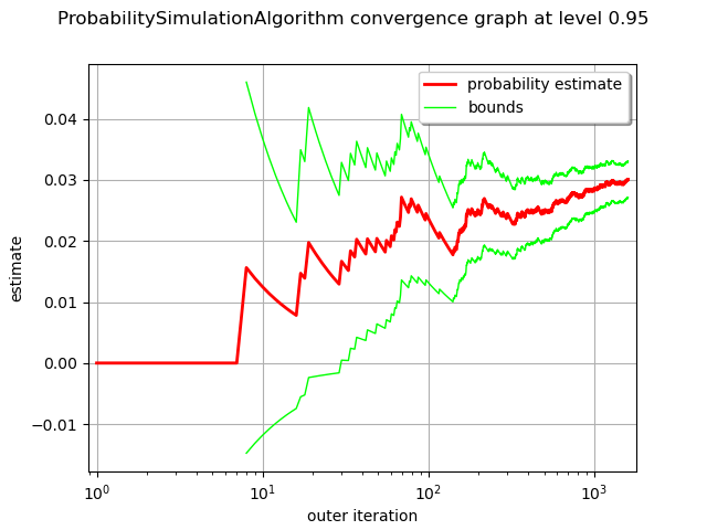
graph = algoMC.drawProbabilityConvergence()
graph.setLogScale(ot.GraphImplementation.LOGX)
view = viewer.View(graph)

Using FORM analysis

We create a NearestPoint algorithm

myCobyla = ot.Cobyla()
# Resolution options:
eps = 1e-3
myCobyla.setMaximumEvaluationNumber(100)
myCobyla.setMaximumAbsoluteError(eps)
myCobyla.setMaximumRelativeError(eps)
myCobyla.setMaximumResidualError(eps)
myCobyla.setMaximumConstraintError(eps)

For statistics about the algorithm

initialNumberOfCall = limitStateFunction.getEvaluationCallsNumber()

We create a FORM algorithm. The first parameter is a NearestPointAlgorithm. The second parameter is an event. The third parameter is a starting point for the design point research.

algoFORM = ot.FORM(myCobyla, myEvent, myDistribution.getMean())

Perform the analysis.

algoFORM.run()

resultFORM = algoFORM.getResult()
numberOfFunctionEvaluationsFORM = limitStateFunction.getEvaluationCallsNumber() - initialNumberOfCall
probabilityFORM = resultFORM.getEventProbability()
print('Number of calls to the limit state =', numberOfFunctionEvaluationsFORM)
print('Pf =', probabilityFORM)

Out:

Number of calls to the limit state = 98
Pf = 0.0299827855823147

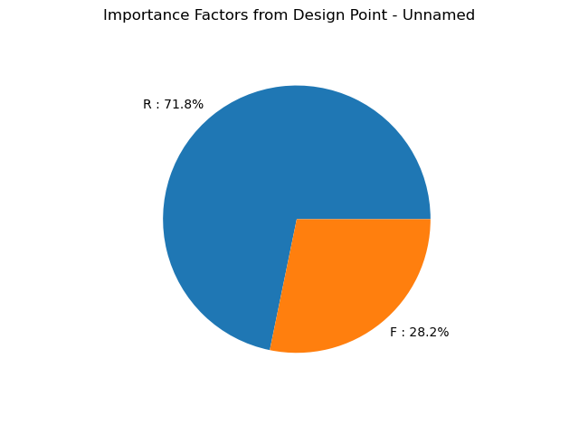
graph = resultFORM.drawImportanceFactors()
view = viewer.View(graph)

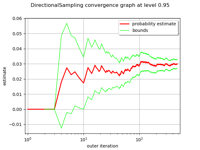
Using Directional sampling

Resolution options:

cv = 0.05
NbSim = 10000

algoDS = ot.DirectionalSampling(myEvent)
algoDS.setMaximumOuterSampling(NbSim)
algoDS.setBlockSize(1)
algoDS.setMaximumCoefficientOfVariation(cv)

For statistics about the algorithm

initialNumberOfCall = limitStateFunction.getEvaluationCallsNumber()

Perform the analysis.

algoDS.run()

result = algoDS.getResult()
probabilityDirectionalSampling = result.getProbabilityEstimate()
numberOfFunctionEvaluationsDirectionalSampling = limitStateFunction.getEvaluationCallsNumber() - initialNumberOfCall
print('Number of calls to the limit state =', numberOfFunctionEvaluationsDirectionalSampling)
print('Pf = ', probabilityDirectionalSampling)
print('CV =', result.getCoefficientOfVariation())

Out:

Number of calls to the limit state = 8832
Pf =  0.02995686422511512
CV = 0.04985883421541657

graph = algoDS.drawProbabilityConvergence()
graph.setLogScale(ot.GraphImplementation.LOGX)
view = viewer.View(graph)

Using importance sampling with FORM design point: FORM-IS

The getStandardSpaceDesignPoint method returns the design point in the U-space.

standardSpaceDesignPoint = resultFORM.getStandardSpaceDesignPoint()
standardSpaceDesignPoint

[-1.59355,0.999463]

The key point is to define the importance distribution in the U-space. To define it, we use a multivariate standard Gaussian and configure it so that the center is equal to the design point in the U-space.

dimension = myDistribution.getDimension()
dimension

Out:

2

myImportance = ot.Normal(dimension)
myImportance.setMean(standardSpaceDesignPoint)
myImportance

Normal(mu = [-1.59355,0.999463], sigma = [1,1], R = [[ 1 0 ]
[ 0 1 ]])

Create the design of experiment corresponding to importance sampling. This generates a WeightedExperiment with weights corresponding to the importance distribution.

experiment = ot.ImportanceSamplingExperiment(myImportance)

Create the standard event corresponding to the event. This transforms the original problem into the U-space, with Gaussian independent marginals.

standardEvent = ot.StandardEvent(myEvent)

We then create the simulation algorithm.

algo = ot.ProbabilitySimulationAlgorithm(standardEvent, experiment)
algo.setMaximumCoefficientOfVariation(cv)
algo.setMaximumOuterSampling(40000)

For statistics about the algorithm

initialNumberOfCall = limitStateFunction.getEvaluationCallsNumber()

algo.run()

retrieve results

result = algo.getResult()
probabilityFORMIS = result.getProbabilityEstimate()
numberOfFunctionEvaluationsFORMIS = limitStateFunction.getEvaluationCallsNumber() - initialNumberOfCall
print('Number of calls to the limit state =', numberOfFunctionEvaluationsFORMIS)
print('Pf = ', probabilityFORMIS)
print('CV =', result.getCoefficientOfVariation())

Out:

Number of calls to the limit state = 872
Pf =  0.02957937670652859
CV = 0.049923000188140665

Conclusion

We now compare the different methods in terms of accuracy and speed.

import numpy as np

The following function computes the number of correct base-10 digits in the computed result compared to the exact result.

def computeLogRelativeError(exact, computed):
    logRelativeError = -np.log10(abs(exact - computed) / abs(exact))
    return logRelativeError

The following function prints the results.

def printMethodSummary(name, computedProbability, numberOfFunctionEvaluations):
    print("---")
    print(name,":")
    print('Number of calls to the limit state =', numberOfFunctionEvaluations)
    print('Pf = ', computedProbability)
    exactProbability = 0.02919819462483051
    logRelativeError = computeLogRelativeError(exactProbability, computedProbability)
    print("Number of correct digits=%.3f" % (logRelativeError))
    performance = logRelativeError/numberOfFunctionEvaluations
    print("Performance=%.2e (correct digits/evaluation)" % (performance))
    return

printMethodSummary("Monte-Carlo", probabilityMonteCarlo, numberOfFunctionEvaluationsMonteCarlo)
printMethodSummary("FORM", probabilityFORM, numberOfFunctionEvaluationsFORM)
printMethodSummary("DirectionalSampling", probabilityDirectionalSampling, numberOfFunctionEvaluationsDirectionalSampling)
printMethodSummary("FORM-IS", probabilityFORMIS, numberOfFunctionEvaluationsFORMIS)

Out:

---
Monte-Carlo :
Number of calls to the limit state = 12837
Pf =  0.030225130482199877
Number of correct digits=1.454
Performance=1.13e-04 (correct digits/evaluation)
---
FORM :
Number of calls to the limit state = 98
Pf =  0.0299827855823147
Number of correct digits=1.571
Performance=1.60e-02 (correct digits/evaluation)
---
DirectionalSampling :
Number of calls to the limit state = 8832
Pf =  0.02995686422511512
Number of correct digits=1.585
Performance=1.79e-04 (correct digits/evaluation)
---
FORM-IS :
Number of calls to the limit state = 872
Pf =  0.02957937670652859
Number of correct digits=1.884
Performance=2.16e-03 (correct digits/evaluation)

We see that all three methods produce the correct probability, but not with the same accuracy. In this case, we have found the correct order of magnitude of the probability, i.e. between one and two correct digits. There is, however, a significant difference in computational performance (measured here by the number of function evaluations).

• The fastest method is the FORM method, which produces more than 1 correct digit with less than 98 function evaluations with a performance equal to (correct digits/evaluation). A practical limitation is that the FORM method does not produce a confidence interval: there is no guarantee that the computed probability is correct.

• The slowest method is Monte-Carlo simulation, which produces more than 1 correct digit with 12806 function evaluations. This is associated with a very slow performance equal to (correct digits/evaluation). The interesting point with the Monte-Carlo simulation is that the method produces a confidence interval.

• The DirectionalSampling method is somewhat in-between the two previous methods.

• The FORM-IS method produces 2 correct digits and has a small number of function evaluations. It has an intermediate performance equal to (correct digits/evaluation). It combines the best of the both worlds: it has the small number of function evaluation of FORM computation and the confidence interval of Monte-Carlo simulation.