Note

Click here to download the full example code

Time variant system reliability problem¶

The objective is to evaluate the outcrossing rate from a safe to a failure domain in a time variant reliability problem.

We consider the following limit state function, defined as the difference between a degrading resistance $r(t) = R - bt$ and a time-varying load $S(t)$ :

..math:: begin{align*} g(t)= r(t) - S(t) = R - bt - S(t) quad forall t in [0,T] end{align*}

The failure domaine is defined by:

$g(t) \leq 0$

which means that the resistance at $t$ is less thant the stress at $t$ .

We propose the following probabilistic model:

$R$ is the initial resistance, and $R \sim \mathcal{N}(\mu_R, \sigma_R)$ ;
$b$ is the deterioration rate of the resistance; it is deterministic;
$S(\omega,t)$ is the time-varying stress, which is modeled by a stationary Gaussian process of mean value $\mu_S$ , standard deviation $\sigma_S$ and a squared exponential covariance model $C(s,t)$ .

The outcrossing rate from the safe to the failure domain at instant $t$ is defined by:

$\nu^+(t) = \lim_{\Delta t \rightarrow 0+} \dfrac{\mathbb{P}\{ g(t) \ge 0 \cap g(t+\Delta t) \leq 0\} }{\Delta t}$

For each $t$ , we note the random variable $Z_t = R - bt - S_t$ where $S_t = S(., t)$ .

To evaluate $\nu^+(t)$ , we need to consider the bivariate random vector $(Z_t, Z_{t+\Delta t})$ .

The event $\{ g(t) \geq 0 \cap g(t+\Delta t) <0\}$ writes as the intersection of both events :

$\mathcal{E}_t^1 = \{ Z_t \geq 0\}$ and
$\mathcal{E}_t^2 = \{ Z_{t+\Delta t} \leq 0\}$ .

The objective is to evaluate:

$\mathbb{P}\{\mathcal{E}_t^1 \cap \mathcal{E}_t^2\} \quad \forall t \in [0,T]$

1. Define some useful functions¶

We define the bivariate random vector $Y_t = (bt + S_t, b(t+\Delta t) + S_{t+\Delta t})$ . Here, $Y_t$ is a bivariate Normal random vector:

whith mean $[bt, b(t+\delta t)]$ and
whith covariance matrix $\Sigma$ defined by:

..math::: begin{align*} Sigma = left( begin{array}{cc} C(t, t) & C(t, t+Delta t) \ C(t, t+Delta t) & C(t+Delta t, t+Delta t) end{array} right) end{align*}

This function buils $Y_t =(Y_t^1, Y_t^2)$ .

def buildNormal(b, t, mu_S, covariance, delta_t = 1e-5):
    sigma = CovarianceMatrix(2)
    sigma[0, 0] = covariance(t, t)[0,0]
    sigma[0, 1] = covariance(t, t+delta_t)[0,0]
    sigma[1, 1] = covariance(t+delta_t, t+delta_t)[0,0]
    return Normal([b*t + mu_S, b*(t+delta_t) + mu_S], sigma)

This function creates the trivariate random vector $(R, Y_t^1, Y_t^2)$ where $R$ is independant from $(Y_t^1, Y_t^2)$ . We need to create this random vector because both events $\mathcal{E}_t^1$ and $\mathcal{E}_t^2$ must be defined from the same random vector!

def buildCrossing(b, t, mu_S, covariance, R, delta_t = 1e-5):
    normal = buildNormal(b, t, mu_S, covariance, delta_t)
    #return BlockIndependentDistribution([R, normal]): only from the 1.16 version!
    marg = [R, normal.getMarginal(0), normal.getMarginal(1)]
    cop = ComposedCopula([IndependentCopula(1), normal.getCopula()])
    return ComposedDistribution(marg, cop)

This function evaluates the probability using the Monte Carlo sampling. It defines the intersection event $\mathcal{E}_t^1 \cap \mathcal{E}_t^2$ .

def computeCrossingProbability_MonteCarlo(b, t, mu_S, covariance, R, delta_t, n_block, n_iter, CoV):
    full = buildCrossing(b, t, mu_S, covariance, R, delta_t)
    X = RandomVector(full)
    f1 = SymbolicFunction(["R", "X1", "X2"], ["X1 - R"])
    e1 = ThresholdEvent(CompositeRandomVector(f1, X), Less(), 0.0)
    f2 = SymbolicFunction(["R", "X1", "X2"], ["X2 - R"])
    e2 = ThresholdEvent(CompositeRandomVector(f2, X), GreaterOrEqual(), 0.0)
    event = IntersectionEvent([e1, e2])
    algo = ProbabilitySimulationAlgorithm(event, MonteCarloExperiment())
    algo.setBlockSize(n_block)
    algo.setMaximumOuterSampling(n_iter)
    algo.setMaximumCoefficientOfVariation(CoV)
    algo.run()
    return algo.getResult().getProbabilityEstimate() / delta_t

This function evaluates the probability using the Low Discrepancy sampling.

def computeCrossingProbability_QMC(b, t, mu_S, covariance, R, delta_t, n_block, n_iter, CoV):
    full = buildCrossing(b, t, mu_S, covariance, R, delta_t)
    X = RandomVector(full)
    f1 = SymbolicFunction(["R", "X1", "X2"], ["X1 - R"])
    e1 = ThresholdEvent(CompositeRandomVector(f1, X), Less(), 0.0)
    f2 = SymbolicFunction(["R", "X1", "X2"], ["X2 - R"])
    e2 = ThresholdEvent(CompositeRandomVector(f2, X), GreaterOrEqual(), 0.0)
    event = IntersectionEvent([e1, e2])
    algo = ProbabilitySimulationAlgorithm(event, LowDiscrepancyExperiment(SobolSequence(X.getDimension()), n_block, False))
    algo.setBlockSize(n_block)
    algo.setMaximumOuterSampling(n_iter)
    algo.setMaximumCoefficientOfVariation(CoV)
    algo.run()
    return algo.getResult().getProbabilityEstimate() / delta_t

This function evaluates the probability using the FORM algorithm for event systems..

def computeCrossingProbability_FORM(b, t, mu_S, covariance, R, delta_t):
    full = buildCrossing(b, t, mu_S, covariance, R, delta_t)
    X = RandomVector(full)
    f1 = SymbolicFunction(["R", "X1", "X2"], ["X1 - R"])
    e1 = ThresholdEvent(CompositeRandomVector(f1, X), Less(), 0.0)
    f2 = SymbolicFunction(["R", "X1", "X2"], ["X2 - R"])
    e2 = ThresholdEvent(CompositeRandomVector(f2, X), GreaterOrEqual(), 0.0)
    event = IntersectionEvent([e1, e2])
    algo = SystemFORM(SQP(), event, X.getMean())
    algo.run()
    return algo.getResult().getEventProbability() / delta_t

2. Evaluate the probability¶

from openturns import *
from openturns.viewer import View
from math import sqrt

First, fix some parameters: $(\mu_R, \sigma_R, \mu_S, \sigma_S, \Delta t, T, b)$ and the covariance model wich is the Squared Exponential model. Be careful to the parameter $\Delta t$ which is of great importance: if it is too small, the simulation methods have problems to converge because the correlation rate is too high between the instants $t$ and $t+\Delta t$ . We advice to take $\Delta t \simeq 10^{-1}$ .

mu_S = 3.0
sigma_S = 0.5
l = 10

b = 0.01

mu_R = 5.0
sigma_R = 0.3
R = Normal(mu_R, sigma_R)

covariance = SquaredExponential([l/sqrt(2)], [sigma_S])

t0 = 0.0
t1 = 50.0
N = 26

# Get all the time steps t
times = RegularGrid(t0, (t1 - t0) / (N - 1.0), N).getVertices()

delta_t = 1e-1

Use all the methods previously described:

Monte Carlo: values in values_MC
Low discrepancy suites: values in values_QMC
FORM: values in values_FORM

values_MC = list()
values_QMC = list()
values_FORM = list()

for tick in times:
    values_MC.append(computeCrossingProbability_MonteCarlo(b, tick[0], mu_S, covariance, R, delta_t, 2**12, 2**3, 1e-2))
    values_QMC.append(computeCrossingProbability_QMC(b, tick[0], mu_S, covariance, R, delta_t, 2**12, 2**3, 1e-2))
    values_FORM.append(computeCrossingProbability_FORM(b, tick[0], mu_S, covariance, R, delta_t))

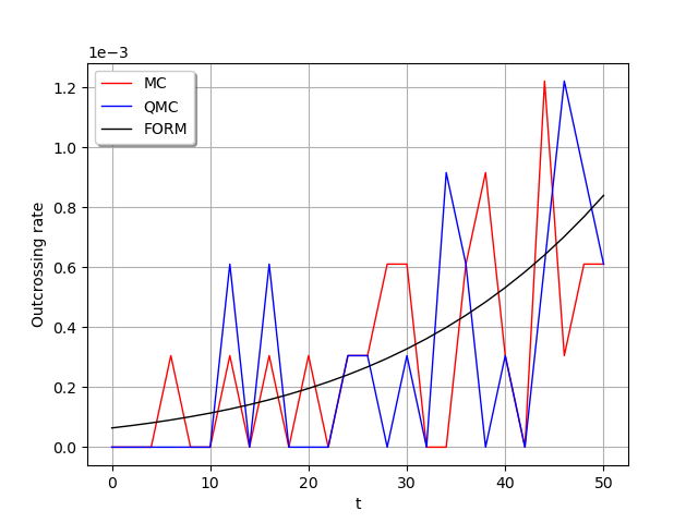
print('Values MC = ', values_MC)
print('Values QMC = ', values_QMC)
print('Values FORM = ', values_FORM)

Out:

Values MC =  [0.0, 0.0, 0.0, 0.00030517578125, 0.0, 0.0, 0.00030517578125, 0.0, 0.00030517578125, 0.0, 0.00030517578125, 0.0, 0.00030517578125, 0.00030517578125, 0.0006103515625, 0.0006103515625, 0.0, 0.0, 0.0006103515625, 0.00091552734375, 0.00030517578125, 0.0, 0.001220703125, 0.00030517578125, 0.0006103515625, 0.0006103515625]
Values QMC =  [0.0, 0.0, 0.0, 0.0, 0.0, 0.0, 0.0006103515625, 0.0, 0.0006103515625, 0.0, 0.0, 0.0, 0.00030517578125, 0.00030517578125, 0.0, 0.00030517578125, 0.0, 0.00091552734375, 0.0006103515625, 0.0, 0.00030517578125, 0.0, 0.0006103515625, 0.001220703125, 0.00091552734375, 0.0006103515625]
Values FORM =  [6.407247221452685e-05, 7.202731340860951e-05, 8.087457491593016e-05, 9.070179169300293e-05, 0.0001016035263802752, 0.00011368175169091608, 0.00012704623305297141, 0.00014181490835112135, 0.00015811426182631293, 0.00017607968850349097, 0.0001958558454373012, 0.00021759698560569734, 0.0002414672698574692, 0.00026764105252706364, 0.0002963031350828803, 0.0003276489830651007, 0.00036188490016252284, 0.00039922815388919713, 0.0004399070467586194, 0.00048416092659680056, 0.0005322401297909951, 0.0005844058510196042, 0.0006409299329987239, 0.0007020945699345352, 0.0007681919182910387, 0.0008395236089949951]

Draw the graphs!

g = Graph()
g.setAxes(True)
g.setGrid(True)
c = Curve(times, [[p] for p in values_MC])
g.add(c)
c = Curve(times, [[p] for p in values_QMC])
g.add(c)
c = Curve(times, [[p] for p in values_FORM])
g.add(c)
g.setLegends(["MC", "QMC", "FORM"])
g.setColors(["red", "blue", 'black'])
g.setLegendPosition("topleft")
g.setXTitle("t")
g.setYTitle("Outcrossing rate")
Show(g)

Total running time of the script: ( 0 minutes 5.927 seconds)

Gallery generated by Sphinx-Gallery

OpenTURNS

An Open source initiative for the Treatment of Uncertainties, Risks'N Statistics

Table of Contents

Previous topic

Next topic

This Page

Time variant system reliability problem¶

1. Define some useful functions¶

2. Evaluate the probability¶